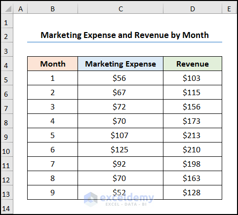
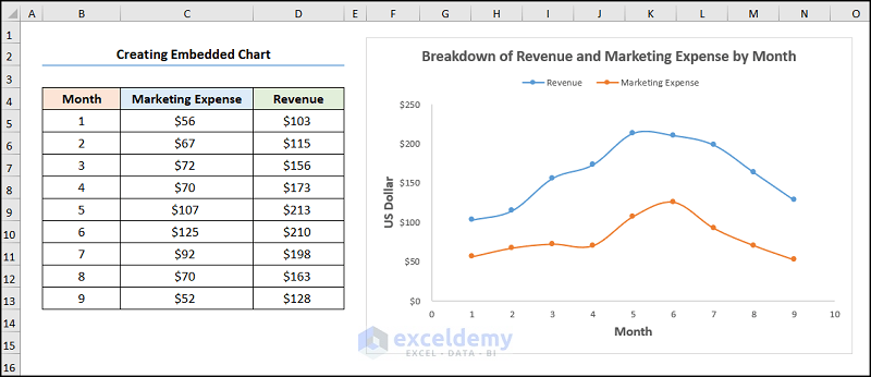
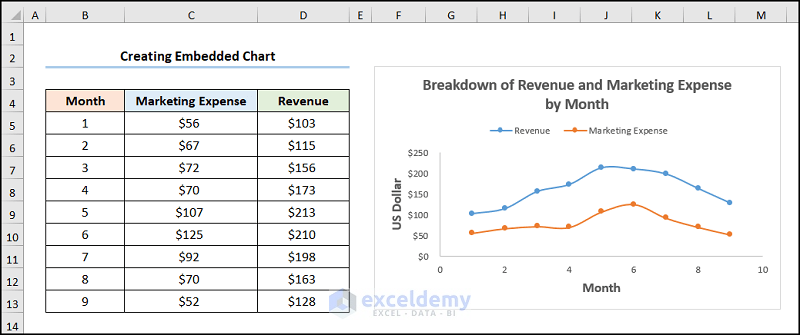
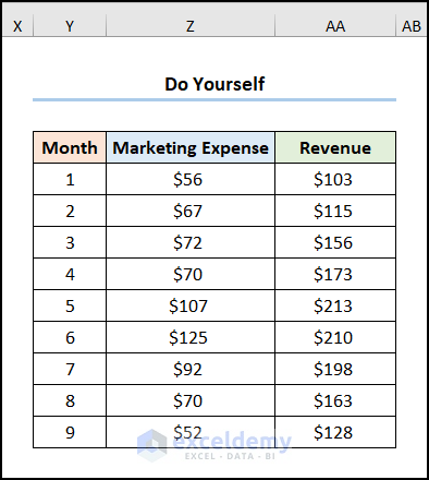
The dataset showcases Month number, Marketing Expense, and the Revenue in USD.
Step 1 – Add a Series to the Chart
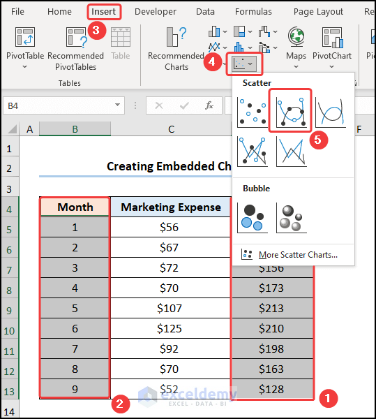
- Select D4:D13 (the Revenue column).
- Hold CTRL and select B4:B13 (the Month column).
- Go to Insert >> click Insert Scatter (X,Y) or Bubble Chart >> choose Scatter with Smooth Lines and Markers.
Step 2 – Add a Second Series to the Chart
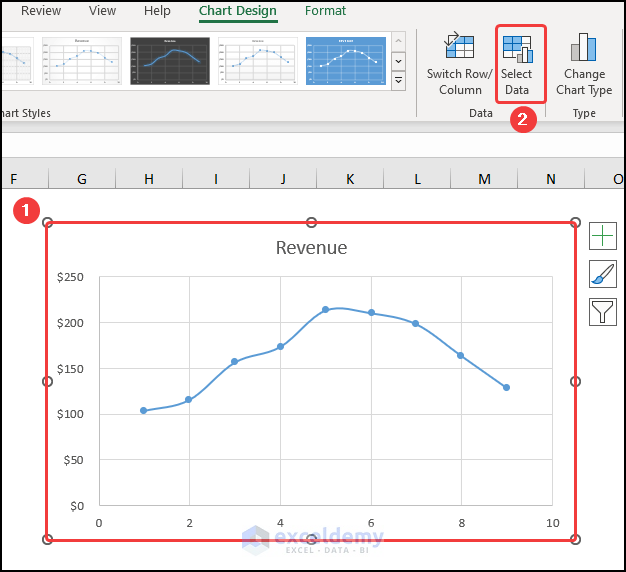
- Select the chart >> choose Select Data in Chart Design.
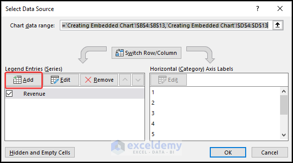
- Click Add to enter a new series.
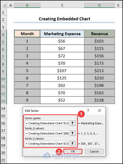
In the Edit Series dialog box.
- Enter the Series name, here, Marketing Expense.
- Choose B5:B13 as Series X values >> select C5:C13 as Series Y values >> Click OK.
Step 3 – Format the Chart
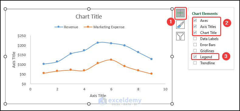
- Go to Chart Elements, enable the Axes Title to name the axes. Here, Month and US Dollar.
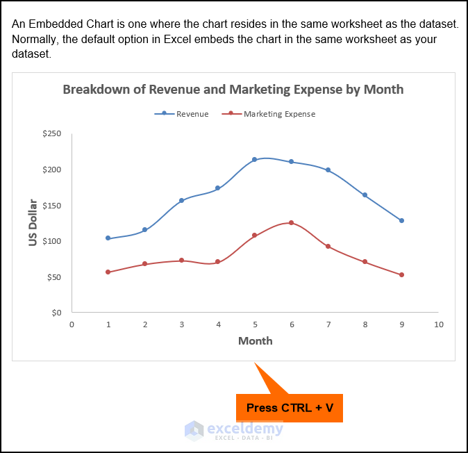
- Add a Chart Title, here, Breakdown of Revenue and Marketing Expense by Month.
- Check Legend to show the two series.
- Uncheck Gridlines.
This is the output.
Moving an Embedded Chart into a Chart Sheet
Steps:
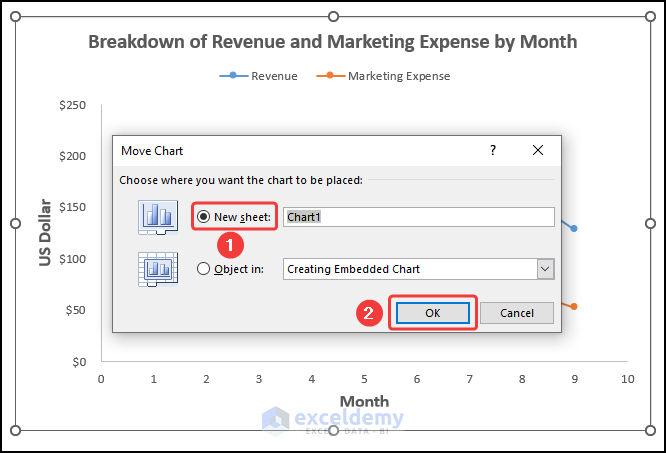
- Select the chart >> go to Chart Design and choose Move Chart.
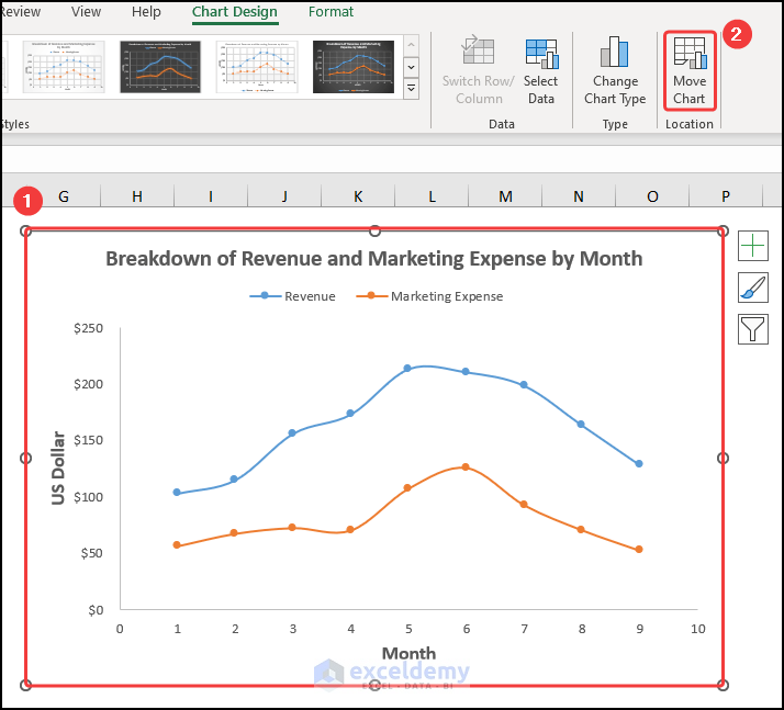
In the Move Chart wizard:
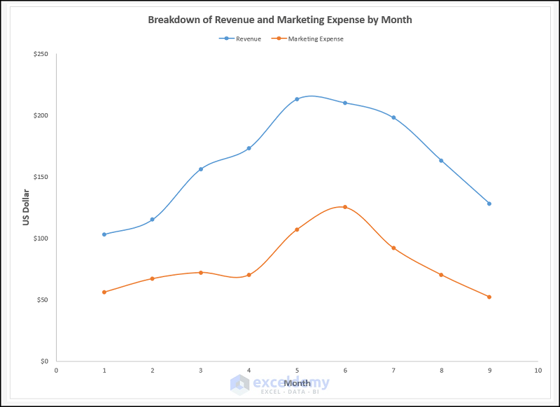
- Select New sheet >> click OK.
This is the output.
Moving a Chart Sheet into an Embedded Chart
Steps:
- Select the chart in the chart sheet >> click Move Chart.
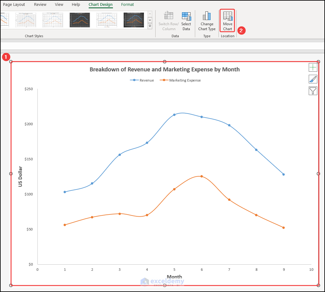
In the Move Chart wizard:
- Select Object in and enter the name of the sheet to insert the chart, here: Creating Embedded Chart.
- Click OK.
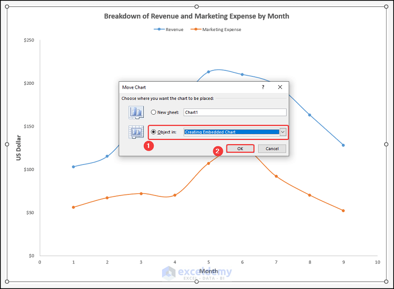
This is the output.
Printing an Embedded Chart
Steps:
- Insert a chart.
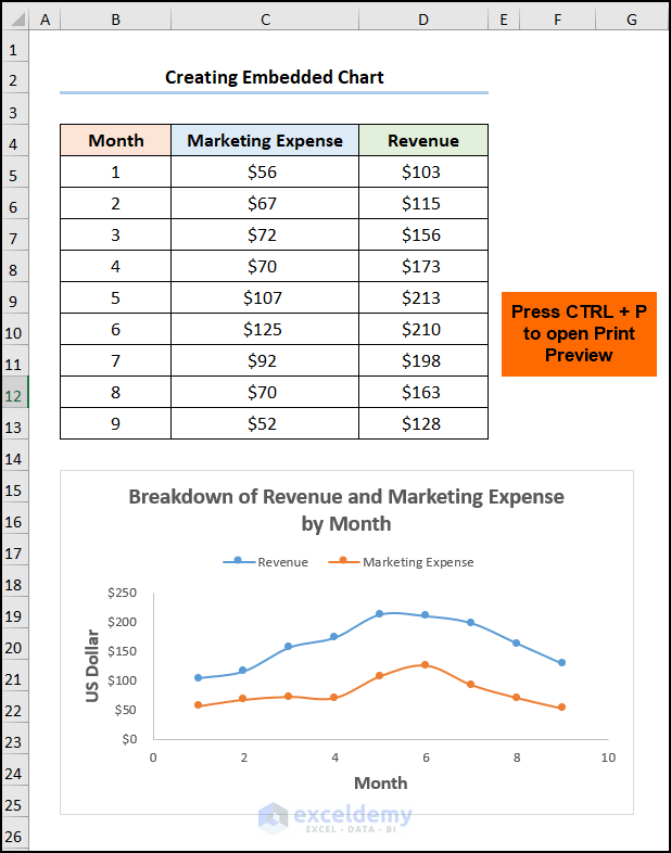
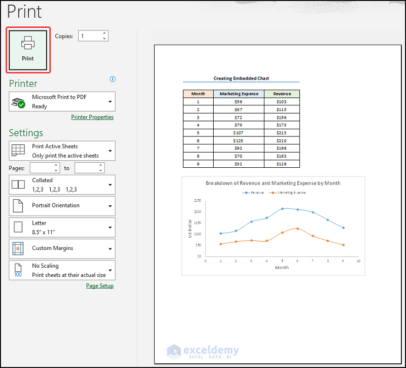
- Press CTRL + P to open print preview.
- Click Print.
Read More: How to Print Graph in Excel
How to Embed an Excel Chart into a Word Document
Steps:
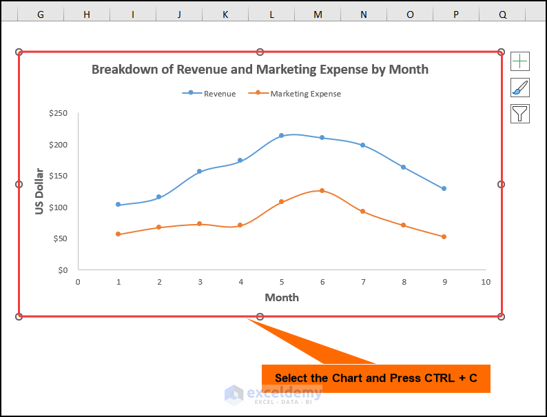
- Select the chart >> press CTRL + C to copy the chart.
- Open a Word document >> choose a location to insert the chart.
- Press CTRL + V to paste it.
Read More: How to Refresh Chart in Excel
Practice Section
Practice here.
Download Practice Workbook
Download the practice workbook.
<< Go Back To Excel Charts | Learn Excel
Get FREE Advanced Excel Exercises with Solutions!

