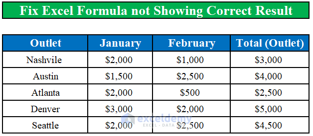
[Fixed!]: Excel Formula Not Showing Correct Result (8 Methods)

We have an Excel worksheet that has the information about the revenues of different outlets of a chain restaurant for January and February. We will use this workbook to show you how to fix an Excel formula not showing the correct result.

Fix 1 – Changing Formula Calculation to Automatic from Manual in Excel

Steps:

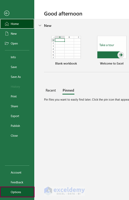
Click on File.

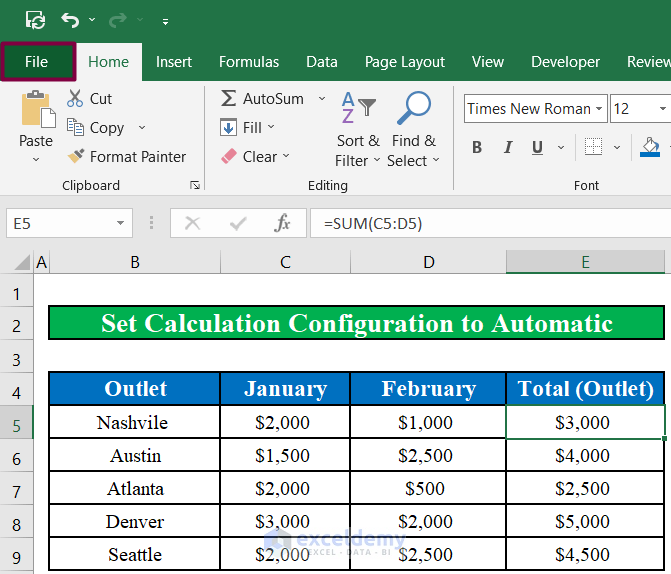
Click on Options.

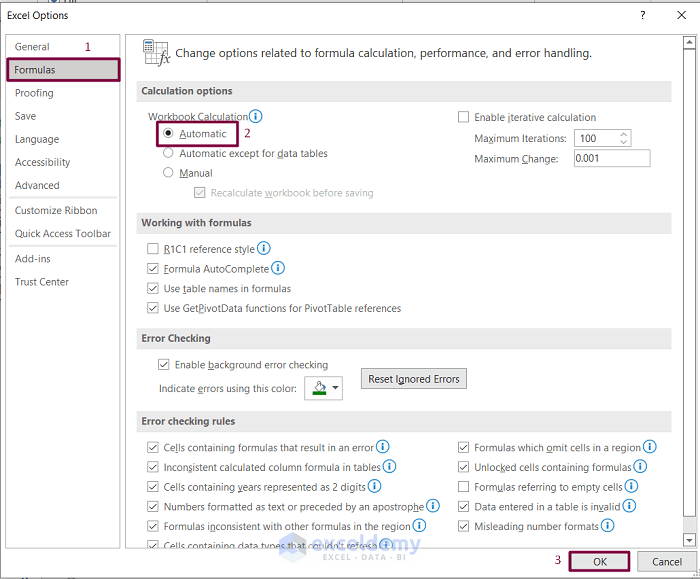
Another window will appear. Click on the Formula tab from the window.
Select Automatic for Workbook Calculation option under the Calculation options
Click on OK.

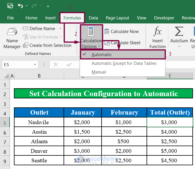
Alternative 1:

Click on the Calculation Options drop-down under Formulas.
Select Automatic from the drop-down list.

Re-Calculating:

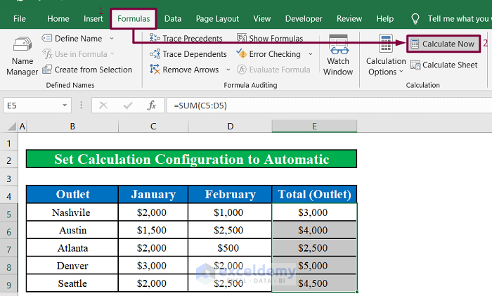
Select all the cells containing the formulas.
Click on Calculate Now under the Formula. The formula will then calculate all the cells and returns the updated result.

Fix 2 – Turning Off the Show Formula Button in Excel to Display the Correct Result

Steps:

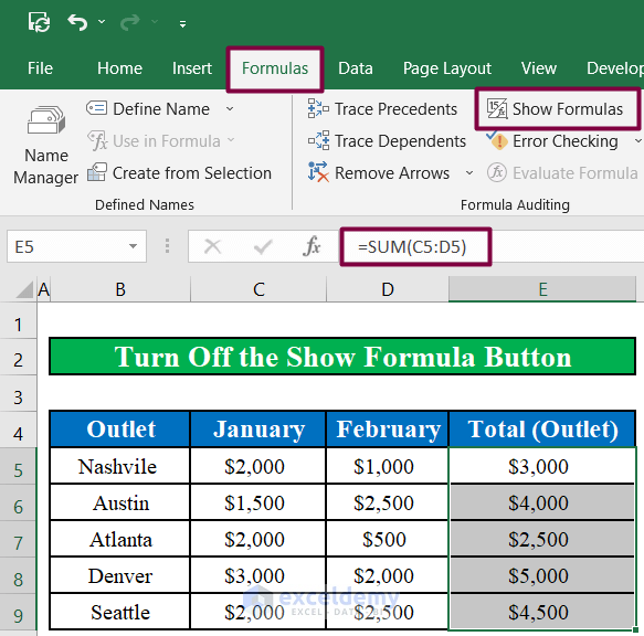
Click on the Show Formulas option under Formulas.

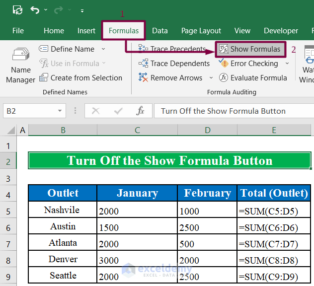
The Show Formulas option is not selected anymore, and the Excel formulas are showing the correct result in the Total (Outlet) column.

Fix 3 – Changing the Format of the Excel Formula to Number from Text

Steps:

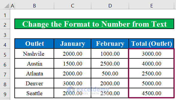
The cells in the Total (Outlet) column are formatted Text instead of Number and the formulas are shown as cell values instead of the results.

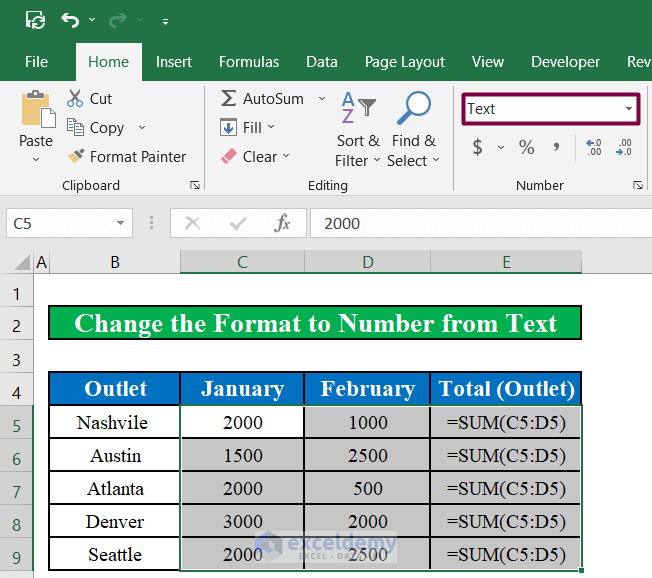
Select all the cells of the January, February, and Total (Outlet) columns.
Change the cell format to Number.

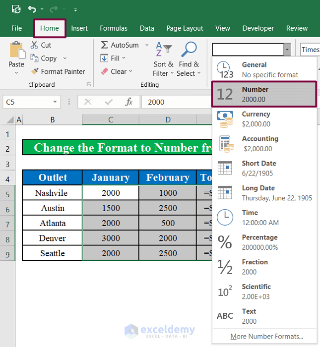
Click on cell E5 and press Enter.

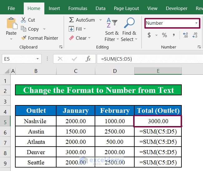
Drag the fill handle down to change the format to number for the rest of the cells in the Total (Outlet) column.

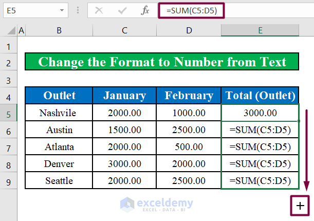
Here’s the result.

Fix 4 – Checking for a Circular Reference in Excel Formula

Steps:

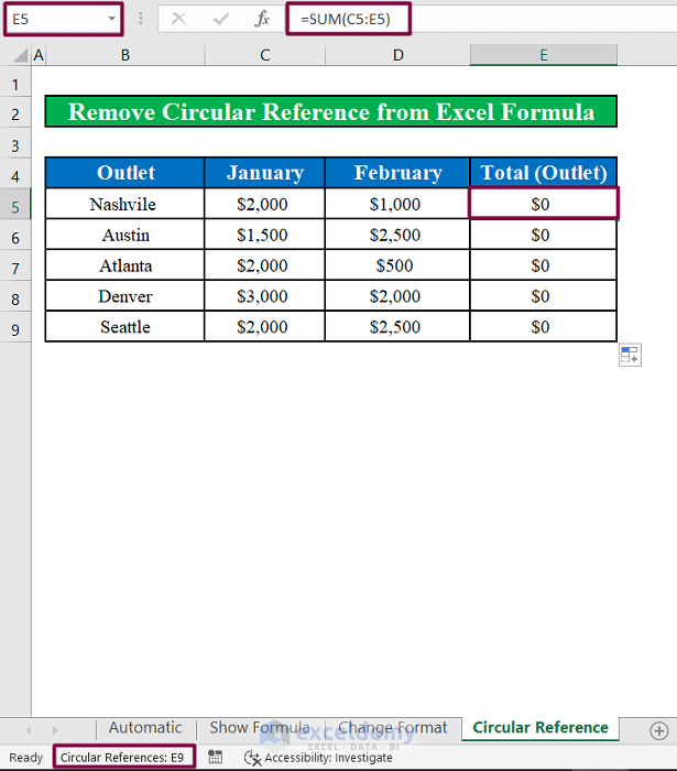
The image below shows that cell E5 in the Total (Outlet) column is showing zero (0) instead of results. The formula in that cell has included the cell itself.
If we look at the sheet tab, we will see that it is showing a circular reference indicating that cell E5 contains a formula that includes the cell itself.

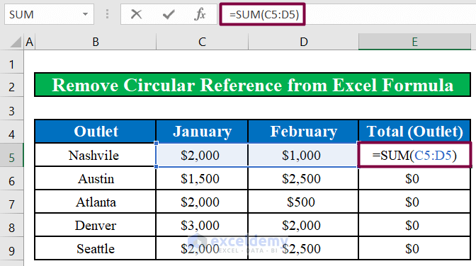
Change the formula to =SUM(C5:D5) to remove the cell E5 from the formula that contains it.

Drag the fill handle down to remove the circular references from each cell in the Total (Outlet) column.

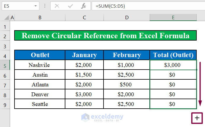
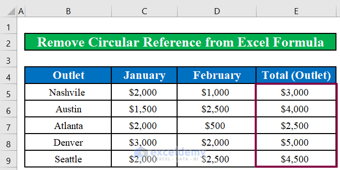
The formula of each of the cells in the column is now showing the correct result.

Fix 5 – Checking If the Equal Sign Is Missing in a Formula

Steps:

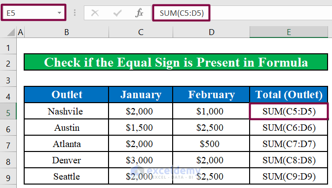
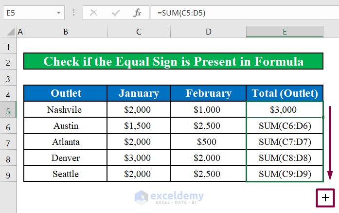
The image below shows that Excel is showing the formula as the cell values in the Total (Outlet) The formulas do not have equal signs in front of them. So, Excel considers them as texts.

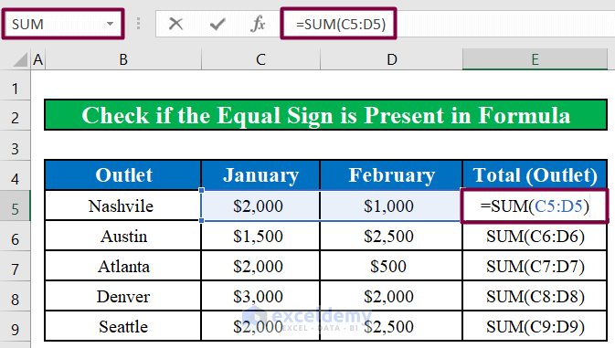
Insert an equal sign (=) in front of the formula in cell E5. The cell references in the SUM formula are colored in blue indicating that formula is working.

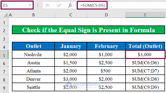
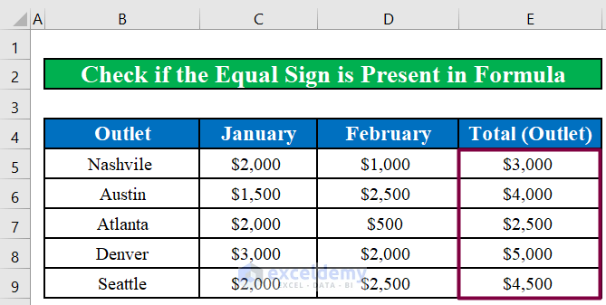
The formula in cell E5 is showing the correct result.

Drag the fill handle down to insert an equal sign (=) in front of each cell in the Total (Outlet).

The formula of each of the cells in the column is now showing the correct result.

Fix 6 – Checking for Hidden Rows or Columns

Steps:

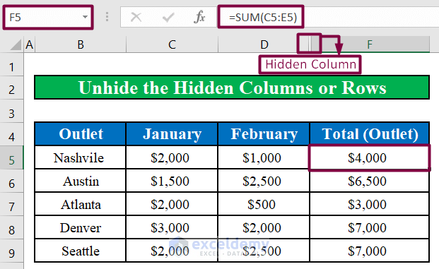
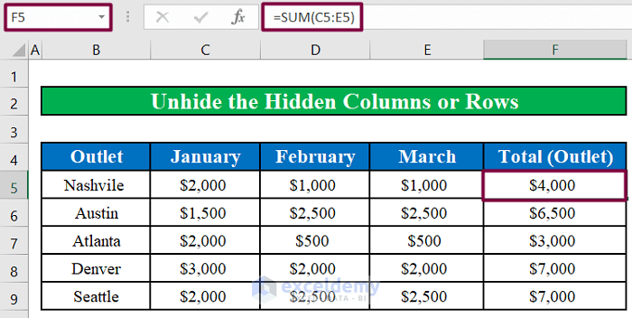
The image below shows that the formulas in the cells under the Total (Outlet) column are not showing the correct result. The formula includes column E but there is no column E in the worksheet as you can see. But if you look carefully, you will see that there is a small gap between columns D and F. The gap indicates that there is a hidden column and that column is column E. We will now unhide column E.

Select columns D and F. Hidden column E is between these two columns.
Go to Home then to Format.
Choose Hide & Unhide and select Unhide Columns.

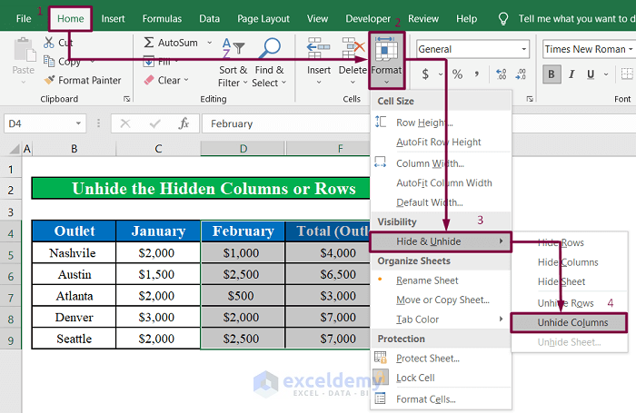
The column E is visible.

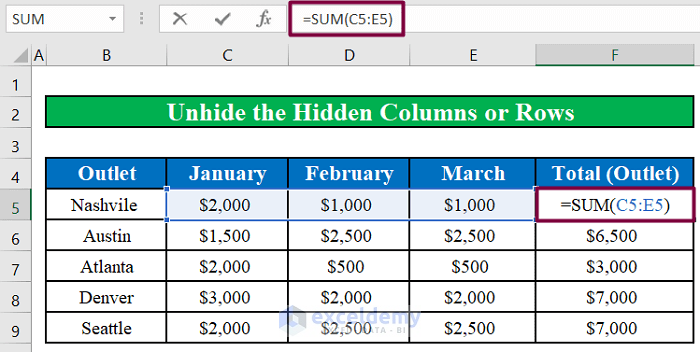
Press Enter, and all the formulas in Total (Outlet) are showing the correct result.

Fix 7 – Checking for Deleted Rows or Columns Leading to the #REF! Error

Steps:

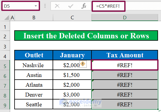
The image below shows that formulas in the Tax Amount column throw #REF! errors as they do not have tax rates to calculate the tax amounts. That happens because we have accidentally deleted the column that has the tax rates.

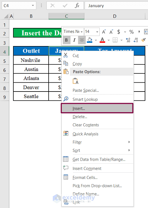
Select cell C5 and right-click on it to bring up the context menu.
Select Insert from that menu.

Another window titled Insert will appear. Select the entire column option from that window.
Click on OK.

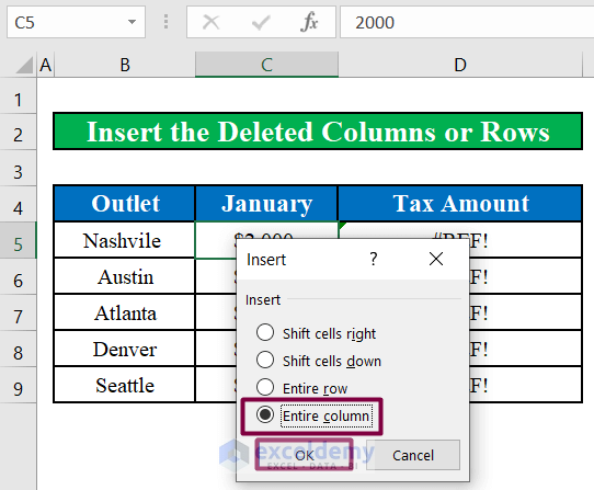
A new column will appear. We will title it Tax Rate.
Rewrite the formula in cell E5 like below.

=C5*D5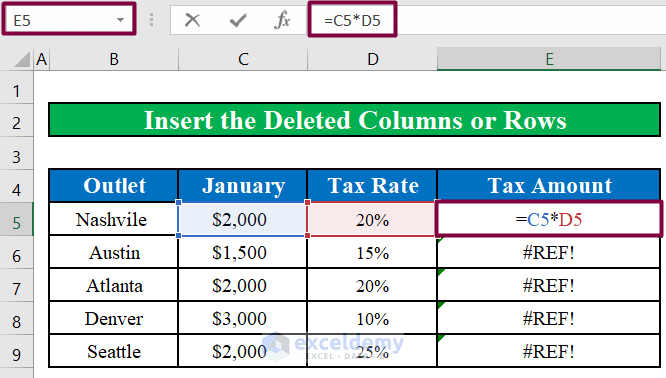

Upon pressing Enter, we will see that the formula in cell E5 is showing the correct result.
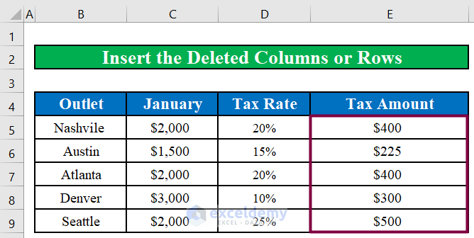
Drag the fill handle down to apply the change to each formula in the Total (Outlet).

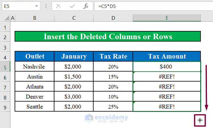
Here’s the result.

Fix 8 – Placing the Parentheses Correctly

Steps:

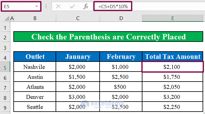
The image below shows that the formula in cell E5 is not showing the correct total tax amount as we did not insert parentheses around the cell references.

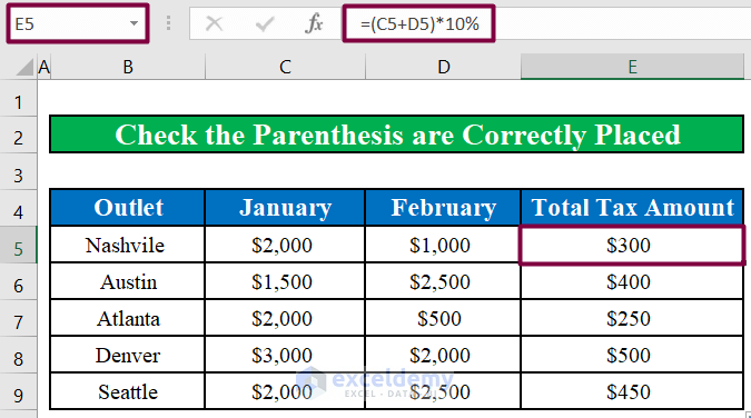
Rewrite the formula like below to insert parentheses around the cell references in the correct way.

=(C5+D5)*10%

Repeat for the rest of the formulas in the Total Tax Amount.

Quick Notes

You should include all the arguments required for a specific formula to calculate the result. You do not have to worry about the optional arguments. A formula still can calculate the result without the optional ones.
While nesting one formula inside another, you should not nest more than 64 functions inside a single formula.
If you enclose a number in double-quotes, Excel will consider it as a text instead of a number.
While entering or inserting numbers in an Excel formula, you should not use any sort of formatting. Remember that, a comma (,) is used in an Excel function to separate the arguments of the function. A dollar sign ($) is used to make a cell reference absolute.
You should separate the arguments of an Excel function with the correct separator. Users in North America should separate the arguments using the comma (,) while those in Europe should do that using the semi-colon (;). Go to Control Panel > Region and Language > Additional Settings which character is set as List Separator and use that character to separate the arguments of a function.
When referring to other worksheets or workbooks with titles that contain spaces or non-alphabetic characters, use single quotation marks around the name of that worksheet or workbooks. Reference to another sheet,

=SUM(‘Tax Calculation’!B2:B10)

Reference to another workbook:

=SUM(‘[Restaurant Sales.xlsx]Tax Calculation’!B2:B10)

When referring to a closed workbook that is closed, you must include the name of that workbook along with the full path of that workbook. For example,

=SUM(‘E:\Reports\[Restaurant Sales.xlsx]Tax Calculation’!B2:B10)

Download the Practice Workbook

Formula Not Showing Correct Result.xlsx