Dataset Overview
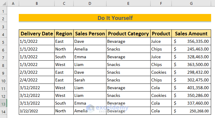
Let’s assume we have a dataset of a company’s sales with columns A to G representing Delivery Date, Region, Sales Person, Product Category, Product, and Sales Amount, respectively.
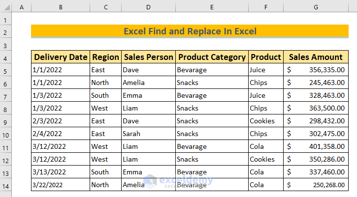
Method1 – Using the Find & Replace Feature
Steps
- Press the keyboard shortcut CTRL + H or navigate to Home, select Editing, choose Find & Select and click on Replace.
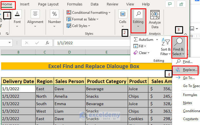
- In Find what box enter the text you want to find for replacement.
- In the Replace with box enter the replacement text (e.g., replace Chips with Crackers).
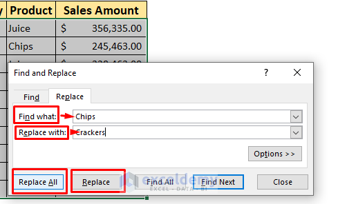
- Choose either Replace All to replace all instances at once or Replace to replace one by one.
- If you select selected Replace All a dialog box will indicate how many replacements were done.
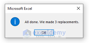
- All the Chips have been Replaced with Crackers.
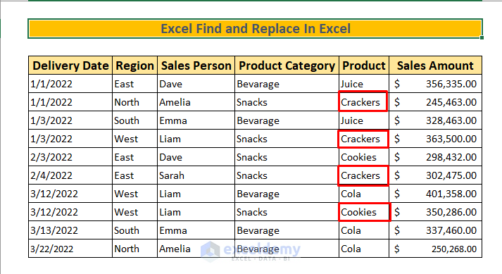
Method 2 – Finding and Replacing Specific Format
Steps
- Open the Find & Replace dialogue box.
- Click on the Options to explore additional settings.
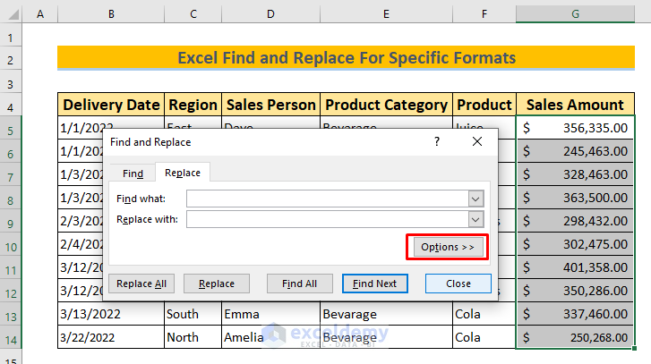
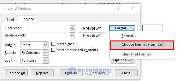
- To find a specific format, click the First Format box and select Choose Format From Cell.
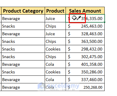
- Pick a cell containing the format you want to find.
- Select the Format you want to Replace.
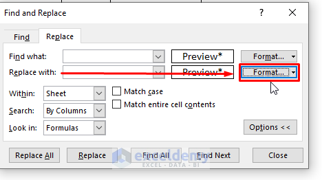
- Click the Format box and choose your desired replacement format (e.g., changing from Accounting Format to Currency Format).
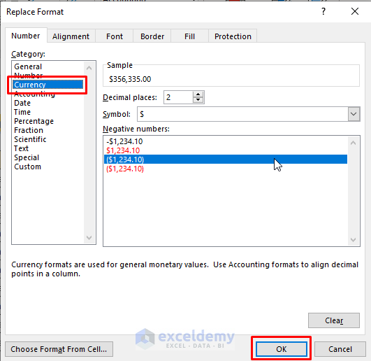
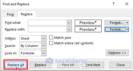
- Press OK and then Replace All.
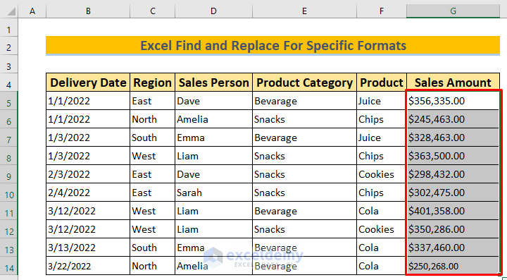
- The selected data has been Replaced with Currency Format.
Read More: How to Find and Replace within Selection in Excel
Method 3 – Replacing Formulas in a Column
Steps
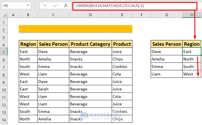
- Suppose you’ve applied the INDEX & MATCH formula in Column H:
- B6:E15 is my data Range for the INDEX function.
- G6 is the reference Cell.
- E6:E15 is the reference Column.
- 0 indicates an exact match, and 1 refers to the first column in the data range.
- This will give you output in column H for corresponding data in Column G.
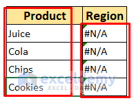
- Change Column I & rename it Product, the formula won’t give any output in the Column Region.
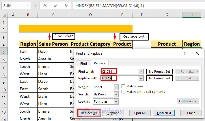
- To modify the formula:
- Go to the Find & Replace dialogue box.
- Enter the necessary changes in the Find What and Replace With boxes.
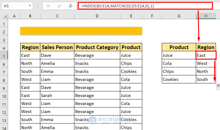
- Press Replace All to update the formula and see the output.
Method 4 – Find and Replace with Nothing
Steps
- Select the column where you want to find and replace data (e.g., the Comment Column in your dataset).
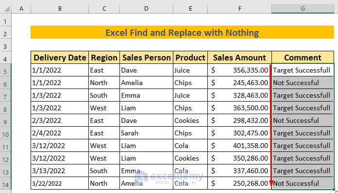
- Open the Find & Replace dialogue box.
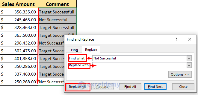
- Enter Not Successful in Find what box.
- Leave the Replace With box empty.
- Click Replace All to remove all instances of Not Successful.
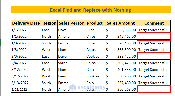
- This will result in the desired data set.
Method 5 – Replacing Line Breaks
Steps
- Select the column with line breaks (e.g., Column G in your dataset).
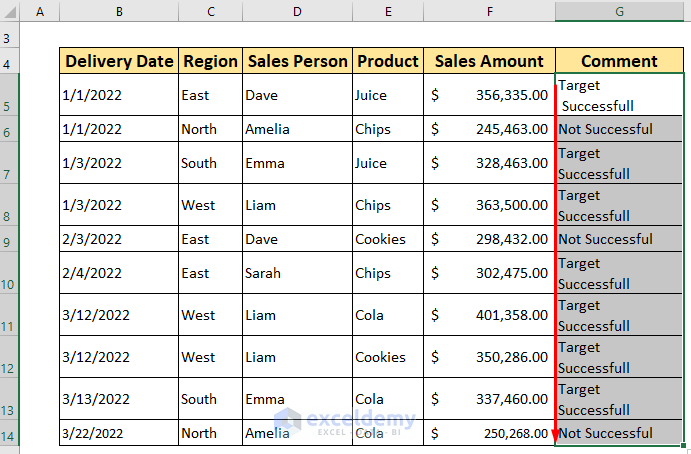
- Open the Find & Replace dialogue box.
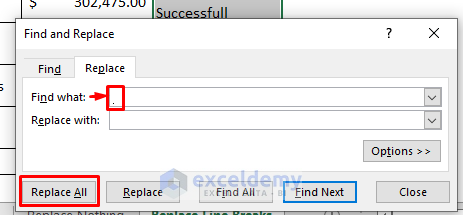
- Enter CTRL+J (represents a line break) in the Find what box.
- Keep the Replace With box empty.
- Click Replace All to replace line breaks.
Method 6 – Using Wildcards for Find and Replace
Steps
- Select the Column where you want to Find & Replace.
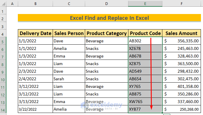
- Open the Find & Replace dialogue box.
- Use Wildcards:
- Asterisk (*) finds and replaces multiple characters (e.g., ab* matches abraham and abram).
- Question mark (?) finds single characters (e.g., P?ter matches both Peter and Piter).
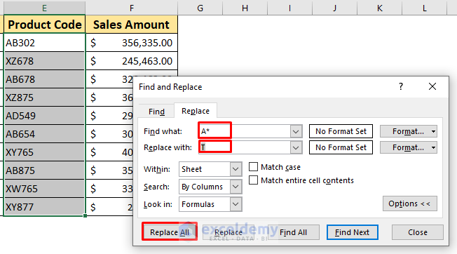
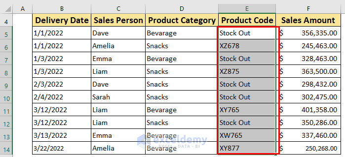
- To find cells with a product code starting with A and replace them with Stock Out:
- Enter A* in Find what box.
- Enter Stock Out in the Replace with box.
- Press Replace All.
- You will have your desired dataset.
Practice Worksheet
Feel free to practice using the provided worksheet.
Download Practice Workbook
You can download the practice workbook from here:
Related Articles
- How to Find and Replace Asterisk (*) Character in Excel
- Find and Replace Tab Character in Excel
- [Fixed!] Excel Find and Replace Not Working
- Find And Replace Multiple Values in Excel
- How to Replace Special Characters in Excel
- How to Substitute Multiple Characters in Excel
<< Go Back to Find and Replace | Learn Excel
Get FREE Advanced Excel Exercises with Solutions!

