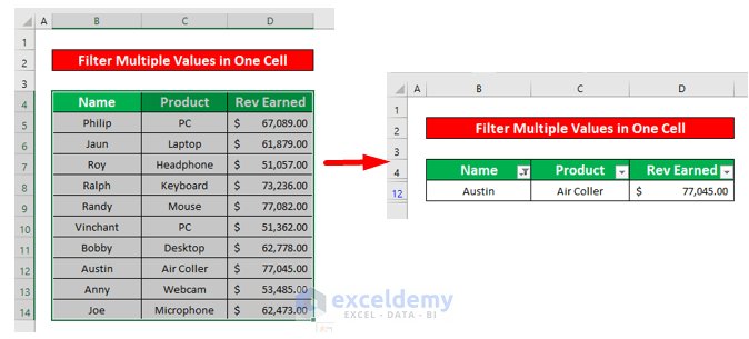
The sample worksheet contains information about several sales representatives of Armani Group. The name of the Products and the Revenue Earned by the sales representatives are given in Columns C and D respectively. We will filter multiple values in one cell in Excel using the Filter Command, Advanced Filter Command, the COUNTIF function, and the FILTER function.
Method 1 – Apply Filter Command to Filter Multiple Values in Excel
Step 1:
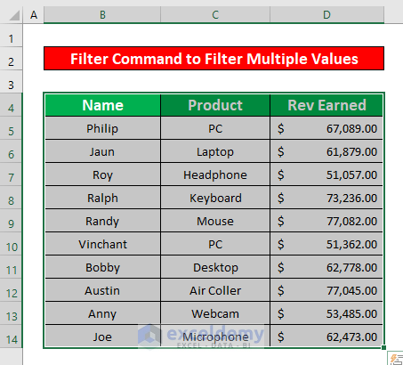
- Select cells array B4 to D14.
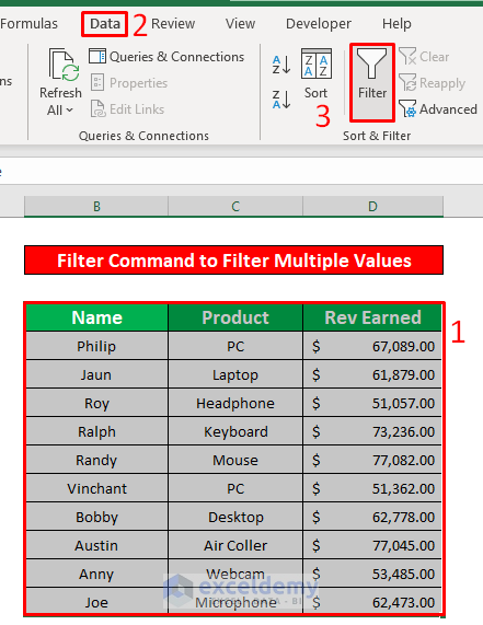
- Select Data on the ribbon and then Filter.
Data → Sort & Filter → Filter
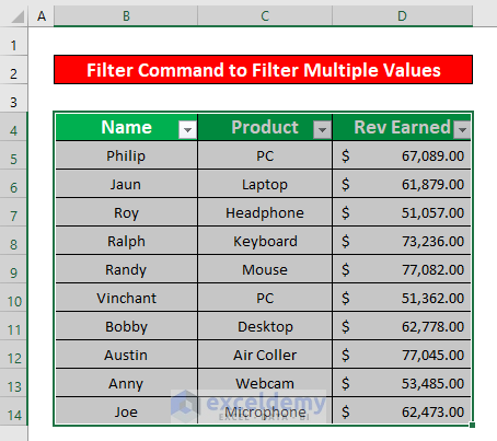
- A filter drop-down will appear in the header of every column.
Step 2:
- Click on the filter drop-down which is situated beside the Name. A new menu pops up. From that menu check the box next to Austin. Press the OK option.
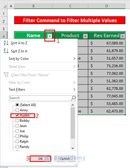
- Only Austin’s information will be visible in the dataset as below.
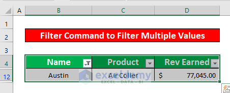
Read More: How to Filter with Multiple Criteria in Excel
Method 2 – Use Advanced Filter Command to Filter Multiple Values in One Cell
Steps:
- Select the relevant cells.
- Select Data on the ribbon and then Advanced in the Sort & Filter options.
Data → Sort & Filter → Advanced
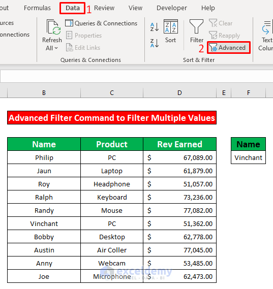
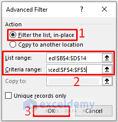
- A dialog box named Advanced Filter will open.
- From the Advanced Filter dialog box, select Filter the list,in-place under the Action.
- Enter the cell range in the List range – in this case the dataset is $B$4:$D$14.
- Enter $F$4:$F$5 as the Criteria range input box.
- Press OK.
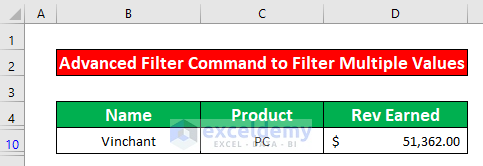
- It is now possible to filter multiple values in one cell as below.
Read More: Excel Filter Data Based on Cell Value
Method 3 – Apply COUNTIF Function to Filter Multiple Values in One Cell
Step 1:
- Select cell E5, and enter the following formula.
=COUNTIF(B5:D14,B5)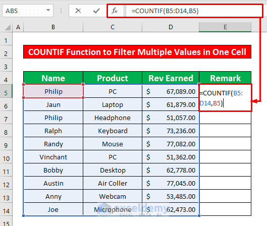
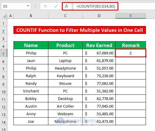
- Press ENTER on the keyboard, and the COUNTIF function will return 2.
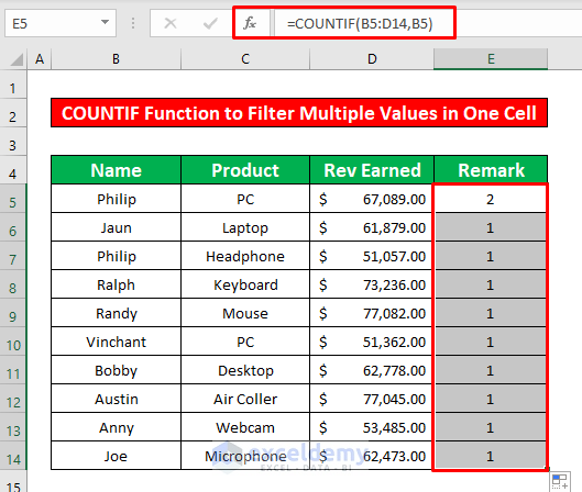
- Drag the AutoFill handle to the rest of the cells in column E.
Step 2:
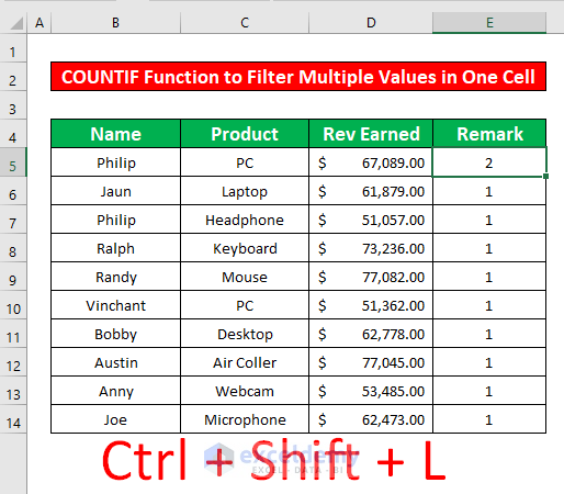
- Press Ctrl + Shift + L simultaneously to create a filter drop-down list.
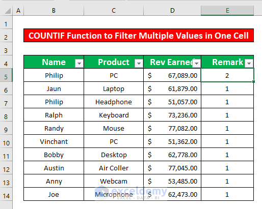
- A filter drop-down list pops up in the header in every column.
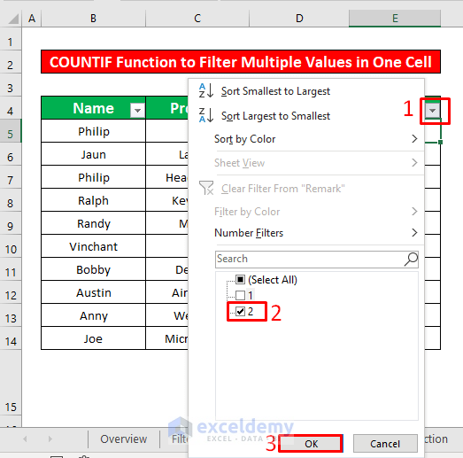
- Click on the filter drop-down beside the Remark heading. A new menu pops up. From that menu check 2.
- Press the OK option.
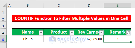
- Philip’s information can now be filtered as below.
Read More: How to Filter Cells with Formulas in Excel
Method 4 – Perform FILTER Function to Filter Multiple Values in Excel
Step 1:
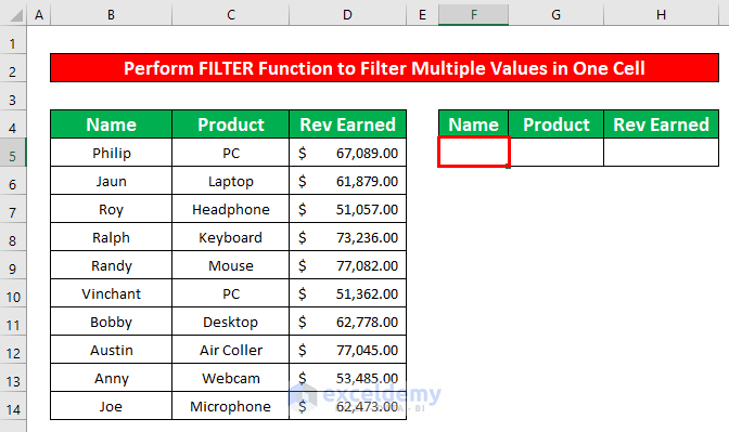
- Create a data table with the same headers as the original dataset.
- Select cell F5.
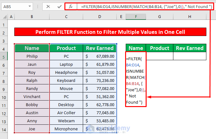
- Enter the below formula.
=FILTER(B4:D14,ISNUMBER(MATCH(B4:B14, {"Joe"},0))," Not Found ")Formula Breakdown:
MATCH(B4:B14, {“Joe”},0)
The MATCH function will match the “Joe” in the cells array B4:D14. 0 indicates an exact match.
ISNUMBER(MATCH(B4:B14, {“Joe”},0))
When a cell contains a number, the ISNUMBER function returns TRUE; otherwise, it returns FALSE.
FILTER(B4:D14,ISNUMBER(MATCH(B4:B14, {“Joe”},0)),” Not Found “)
Inside the FILTER function, B4:D14 is the cells filtering array, ISNUMBER(MATCH(B4:B14, {“Joe”},0)) works like a Boolean array; it carries the condition or criteria for filtering.
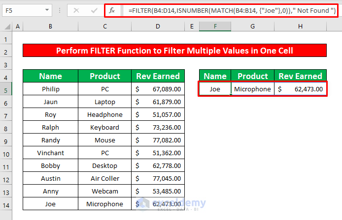
- Press Enter to return the result.
Read More: How to Perform Custom Filter in Excel
Download Practice Workbook
<< Go Back to Data | Filter in Excel | Learn Excel
Get FREE Advanced Excel Exercises with Solutions!

