The Excel Sort option allows us to customize the order of worksheet data. We can sort data alphabetically, numerically, date-wise, etc. Let’s explore some examples.
Method 1 – Using Ascending Order
Suppose we have the below dataset, containing several people’s names and their ages.
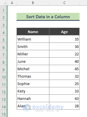
Let’s sort the ages of the above people first, then their names too.
Steps:
- Select the age values of column C.
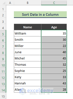
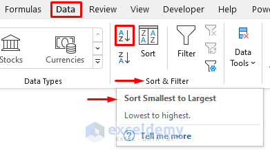
- To sort in ascending order, go to the Data > A to Z icon from the Sort and Filter section.
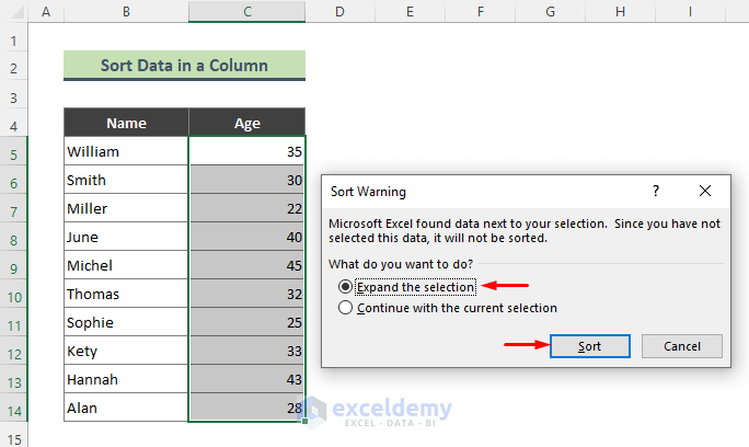
The Sort Warning dialog will appear.
- Select Expand the selection to organize the names of the people according to sorted age.
- Click SORT.
- If you do not want sorting the data in the selected column to affect the rest of the data, then select Continue with the current selection.
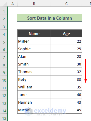
The age values of the people are sorted in ascending order.
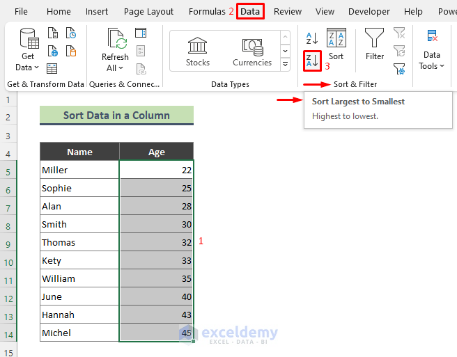
- Similarly, you can organize the above age data in descending order by clicking the Data > Z to A icon.
⏩ Note:
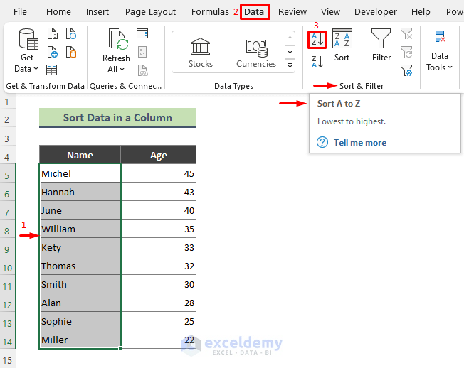
You can sort the names of column B in alphabetical descending/ascending order as follows:
Steps:
- Select the names first.
- Click on the Data > A to Z/ Z to A icon.
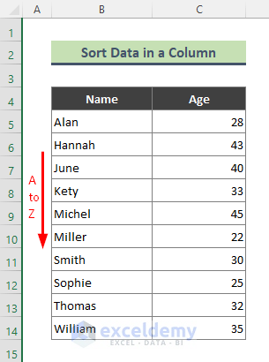
Sorted data is returned. This process can be applied to organize date values too.
Read More: How to Sort Data in Alphabetical Order in Excel
Method 2 – Sorting an Excel Range or Table
Consider the below dataset containing several people’s names, ages, occupations, and cities.
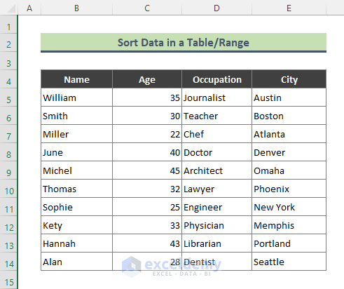
Let’s organize the data in ascending order based on the people’s names.
Steps:
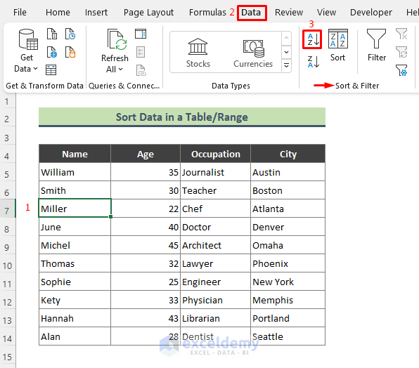
- Select any cell in the column that you want to sort (here, Cell B7).
- Click the Data > A to Z icon.
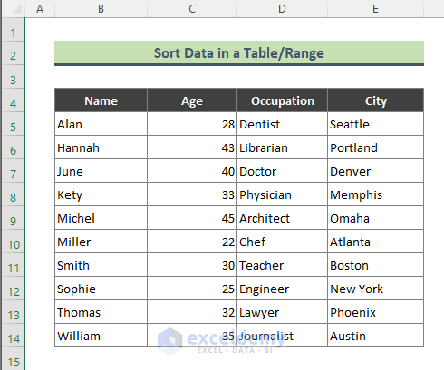
All the name data in column B are sorted, which updates the order of the data in the rest of the columns.
Read More: How to Add Sort Button in Excel
Method 3 – Using Custom Sort
We can use the Custom Sort option to make a custom list and sort data in multiple columns according to it.
3.1 – Sorting Data in Multiple Columns
Steps:
- Select any of the cells in the below dataset.
- Go to Data > Sort.
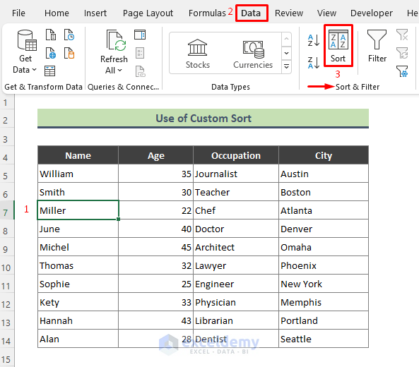
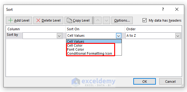
The Sort dialog pops up.
- For the first level, select the column name from the Sort by drop-down.
- Click on Add Level. As we want to add two more levels, we click Add Level twice.
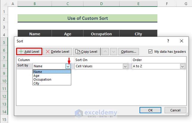
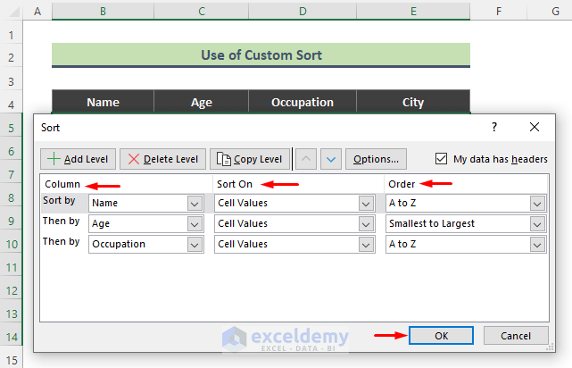
The below levels are added in the Sort dialog.
- Select the columns you want to sort.
- Check Sort On and Order.
- Click OK.
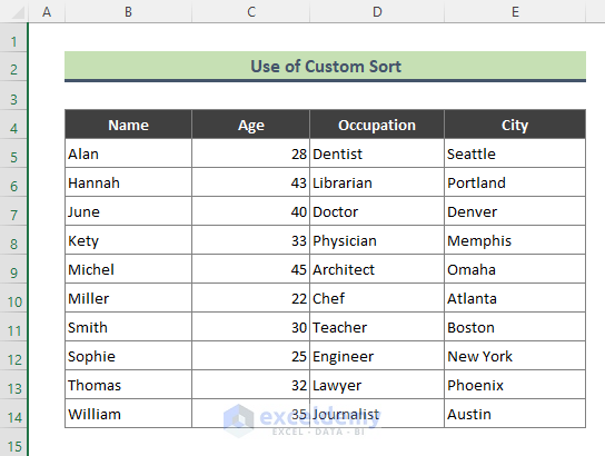
The result is as follows:
Read More: How to Remove Sort by Color in Excel
3.2 – Using a Custom List
Let’s make a custom list and sort values based on it.
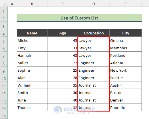
In the below dataset 3 different occupations are listed. Let’s sort the Occupation column according to the list: Lawyer, Engineer, Journalist.
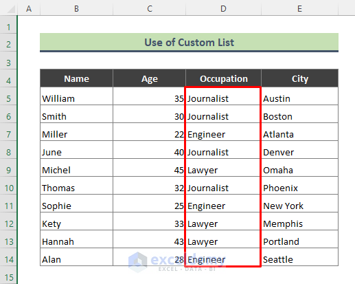
Steps:
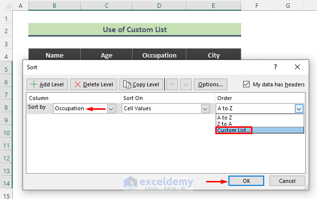
- Select any of the cells from your dataset and go to Data > Sort to open the Sort dialog box.
- In the Sort dialog, click on the Order drop-down and select the Custom List option.
- Press OK.
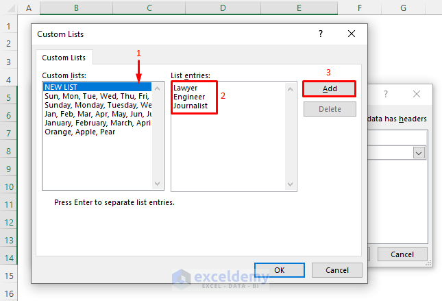
The Custom List dialog appears,
- Click on New List.
- Enter the list items in the List entries box.
- Click Add.
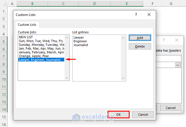
- After the list is added to the Custom List, click OK to close the window.
- In the Sort dialog, click OK to apply the custom list in the Occupation column.
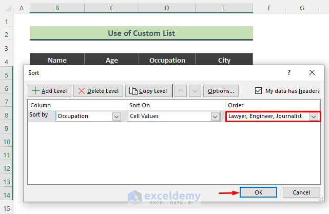
All the data are sorted by the list: Lawyer, Engineer, Journalist.
Read More: Excel Sort and Ignore Blanks
Method 4 – Using SORT Function
If you are using Excel 365/Excel 2021, you can sort data very quickly using this function.
Steps:
- Enter the below formula in Cell E5 and press Enter:
=SORT(B5:C14,2)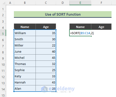
The below result is returned in an array.
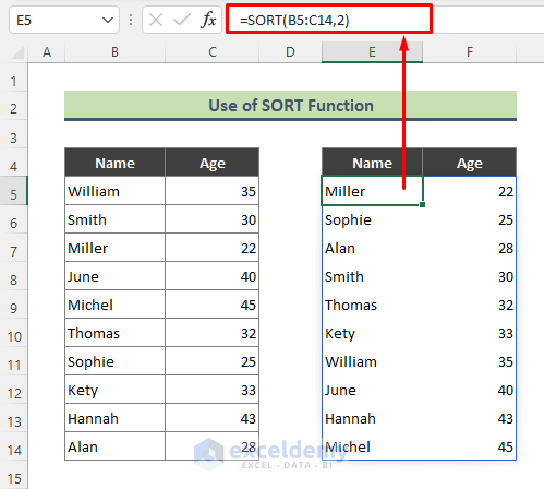
Here, the SORT function orders data in range B5:C14 by column 2.
Read More: How to Sort Data Using Excel Formula
Method 5 – Combining INDEX, MATCH & SMALL Functions to Sort by Numerical Value
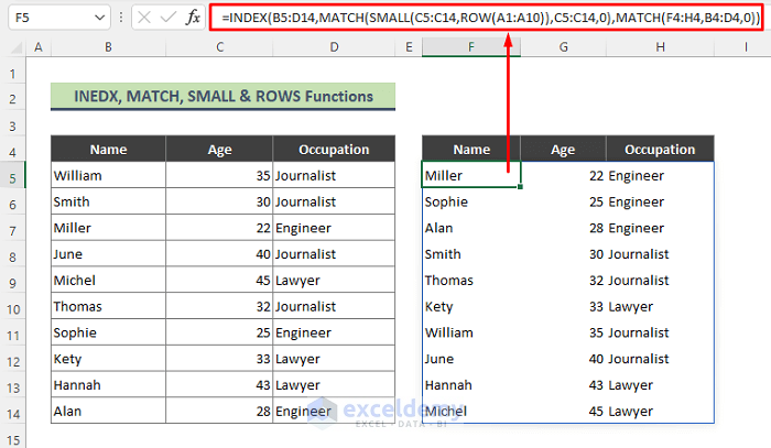
Let’s order people’s names in the below dataset according to their corresponding ages.
Steps:
- Enter the following formula in Cell F5 and hit Enter:
=INDEX(B5:D14,MATCH(SMALL(C5:C14,ROW(A1:A10)),C5:C14,0),MATCH(F4:H4,B4:D4,0))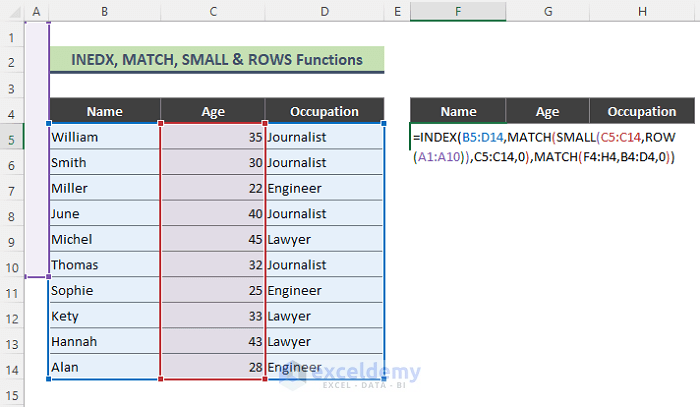
Excel returns the result in the below array. All the age values are sorted in ascending order.
How Does the Formula Work?
- ROW(A1:A10)
The ROW function returns the row number in the range A1:A10 which is:
{1;2;3;4;5;6;7;8;9;10}
- SMALL(C5:C14,ROW(A1:A10))
The SMALL function returns the k-th smallest values in the range C5:C14 as:
{22;25;28;30;32;33;35;40;43;45}
- MATCH(SMALL(C5:C14,ROW(A1:A10))
The MATCH function returns:
{3;7;10;2;6;8;1;4;9;5}
- MATCH(F4:H4,B4:D4,0)
Which resolves to:
{1,2,3}
- INDEX(B5:D14,MATCH(SMALL(C5:C14,ROW(A1:A10)),C5:C14,0),MATCH(F4:H4,B4:D4,0))
Lastly, the INDEX function returns the below result:
{Miller}
Read More: How to Undo Sort in Excel
Things to Remember
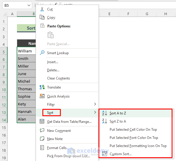
- We can access the Sort option by right-clicking the cell value.
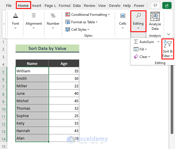
- Alternatively, you will find the Sort option by following the path Home > Editing group > Sort & Filter.
Download Practice Workbook
Further Readings
<< Go Back to Sort in Excel | Learn Excel
Get FREE Advanced Excel Exercises with Solutions!

