How to Use Random 5 Digit Number Generator in Excel (7 Methods)

Method 1 – Using the Excel RANDBETWEEN Function 

Steps:

• Enter the below formula in Cell B5 and press Enter.

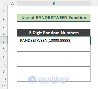
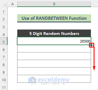
• We will get the below 5-digit number.
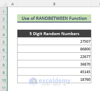
• Use the Fill Handle (+) tool to get 5-digit numbers over B6:B10.

We will get the below output.

⏩ Note:

The RANDBETWEEN function is a volatile function. Random numbers generated by this function change every time a cell on the worksheet is calculated. If you want to avoid these changes in numbers,

• Enter the random numbers generated by the RANDBETWEEN formula by following Home > Copy or Ctrl + C.

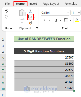
• Paste them as Values by following Home > Paste > Paste Values (see screenshot).

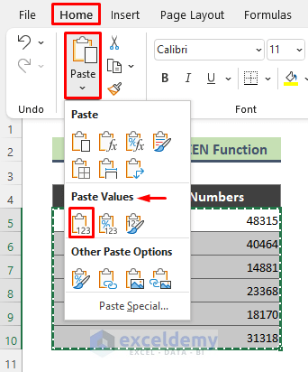
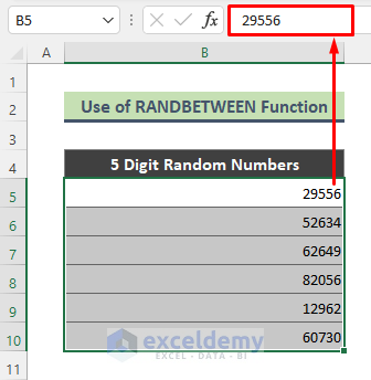
• You will get the numbers as values.

Method 2 – Using LEFT & RANDBETWEEN Functions

Steps:

• Enter the below formula in Cell B6 and hit Enter. The formula will return an empty cell.

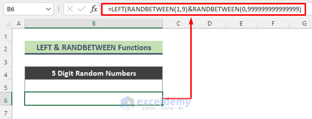
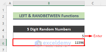
• Enter 5 in Cell B5 as you need a random number with 5 digits.
• Press Enter. You will get a 5-digit random number.

Formula Breakdown

• RANDBETWEEN(1,9)

Here, the above formula returns a random number between 1 and 9.

• RANDBETWEEN(0,999999999999999)

Here, the RANDBETWEEN function returns a random number between 0 and 999999999999999.

• LEFT(RANDBETWEEN(1,9)&RANDBETWEEN(0,999999999999999)&RANDBETWEEN(0,999999999999999),B5

Lastly, the above formula returns a random number containing the length of Cell B5.

Method 3 – Using ROUND & RAND Functions in Excel.

Steps:

• Enter the below formula in Cell B5 and press Enter.

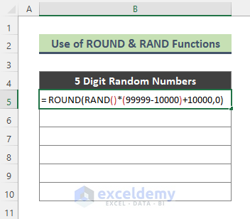
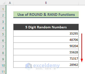
• You will see the below 5-digit numbers.

Formula Breakdown

• RAND()

Here, the RAND function generates random decimal numbers.

• RAND()*(99999-10000)+10000

In this part, the result of the RAND function is multiplied by 89999 and then added to 1000.

• ROUND(RAND()*(99999-10000)+10000,0)

Finally, the ROUND function rounds the result of the previous formula to zero decimal places.

Method 4 – Using Combine INT & RAND Functions

Steps:

• Enter the below formula in Cell B5 and press Enter.

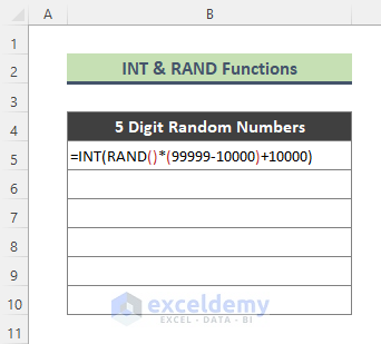
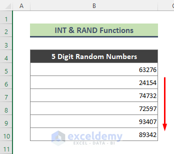
• You will get the following output.

Formula Breakdown

Here, the above formula works similarly to Method 3. The RAND function generates random decimal numbers. The resulting decimal number is multiplied by 89999 and added to 1000. Lastly, the INT function rounds the number to the nearest 5-digit integer.

Method 5 – Using the RANDARRAY Function

Steps:

• Enter the following formula in Cell B5:

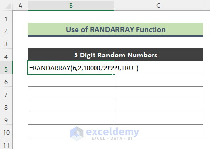
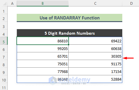
• Press Enter. The above formula returns 5-digit random numbers (integers) over columns B & C and rows 5:10.

Method 6 – Using the Analysis ToolPak 

Steps:

• Go to the File tab from the ribbon.

• Select Options.

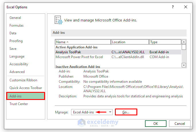
• The Excel Options dialog will appear.
• Click on Add-ins.
• Check Excel Add-ins selected from the Manage drop-down menu and press Go.

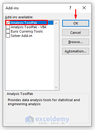
• The Add-ins dialog will open.
• Check on Analysis ToolPak and press OK.

• Go to the Data tab, and the Data Analysis option will open. Click on it.

• The Data Analysis dialog box appears.
• Select Random Number Generation from the Analysis Tools list, and press OK.

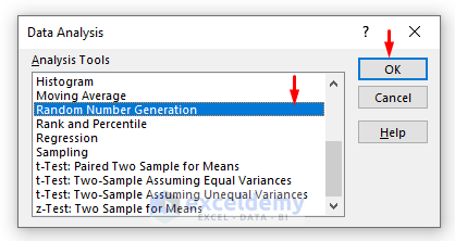
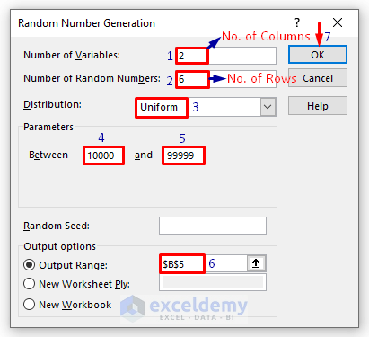
• Enter 2 as the Number of Variables and 6 as the Number of Random Numbers.
• Choose Uniform from the Distribution drop-down. In the Parameters section, enter the range of 5-digit numbers (10000 and 99999) in the Between field.
• Select the Output Range and choose the destination cell (here, cell $B$5).
• Press OK to close the dialog.

• We can see the output below.

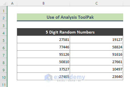
⏩ Note: The 5-digit random numbers generated by Analysis ToolPak contain decimals. To convert those numbers to zero decimal places, you can use the ROUND or INT functions (described in Methods 4 and 5).

Method 7 – Using Excel VBA 

Steps:

• Go to the sheet where you want to get the 5-digit random numbers.
• Right-click on the sheet name and select View Code to bring up the VBA window.

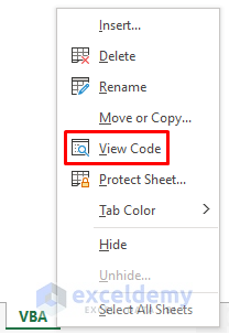
• Enter the below code in the Module and run it using F5.

Sub Random5DigitNumber()
Dim N As Integer
For N = 5 To 10
    ActiveSheet.Cells(N, 2) = Round(Rnd() * (99999 - 10000) + 10000, 0)
Next N
End Sub

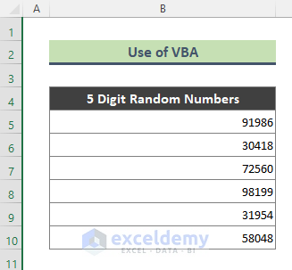
• You will get the below 5-digit numbers.

Things to Remember

• The result we receive from the RANDBETWEEN function contains duplicates. To detect the duplicate numbers, you can use the RANK.EQ function in Excel.
• The RAND function is also a volatile function. You can convert the results returned by the RAND formula to values using the Paste Special option.

Download the Practice Workbook

You can download the workbook to practice.

<< Go Back to Random Number in Excel | Randomize in Excel | Learn Excel