Method 1 – Combine FILTER, ISNUMBER, and SEARCH Functions to Create a Searchable Database in Excel
Step 1:
- Select cell E5 in the sheet named Filter.

- After selecting cell E5, write down the following formulas in the selected cell. The formulas are,
=FILTER(B5:B16,ISNUMBER(SEARCH(Database!B4,B5:B16)),"Not Found")- The SEARCH function in the formula searches for a given value.
- The ISNUMBER function returns True if the output of the SEARCH function is a number. It returns False.
- The FILTER function filters data according to the given criteria.
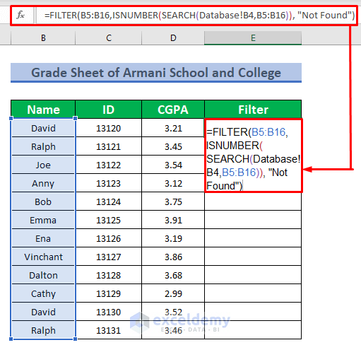
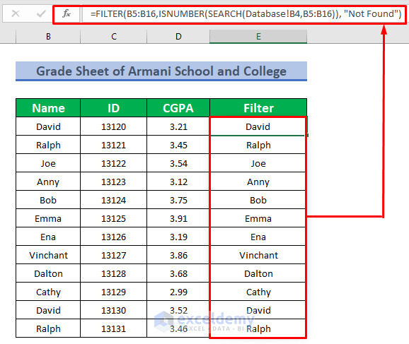
- Press ENTER on your keyboard and you will get your desired output.
Step 2:
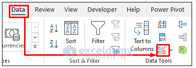
- Select cell B4 in the worksheet named Database. Next, go to,
Data → Data Tools → Data Validation
- Select the Setting tab in the Data Validation dialog box. Choose List in the Allow: field using the drop-down arrow.
- Enter the following formula into the Source typing box.
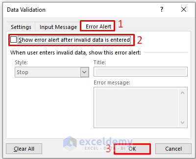
=Filter!$E$5#- Go to the Error Alert tab.
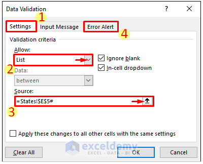
- Uncheck Show error alert after invalid data is entered. Hit OK.
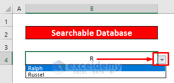
- A searchable database was created. Type something (R) in cell B4. Select the dropdown arrow visible at the lower right corner of the cell. See all the relevant search results as shown in the following screenshot.
2. Run a VBA Code to Create a Searchable Database in Excel
Now, suppose you don’t want to select any dropdown arrow to see the relevant results. Rather you want to see the search results as shown in Google Search. Then follow the steps below.
Step 1:
- First, you need to follow the steps before Data → Data Tools → Data Validation only in the earlier method.
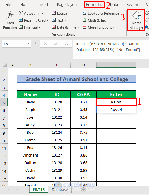
- Then select cell E5 in the Filter. After that, select Formulas → Name Manager.
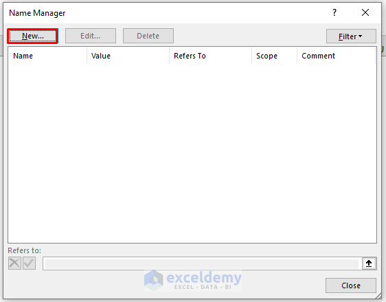
- Next, select New in the Name Manager window.
- Then change the Name to Searchable_Database in the New Name window.
- After that enter the following formula in the Refers to the field. Then hit OK. The formula uses the INDEX and COUNTIF functions.
=Filter!$E$5:$E$5:INDEX(States!$E$5:$E$17,COUNTIF(States!$E$5:$E$17,"?*"))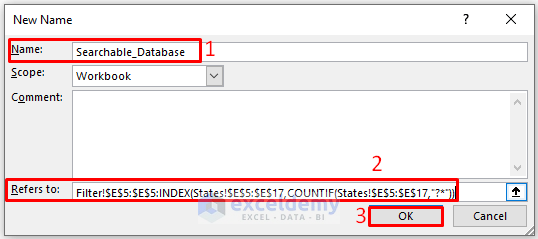
Step 2:
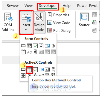
- Now go to the Dropdown sheet. Then select Insert → Combo Box from the Developer tab.
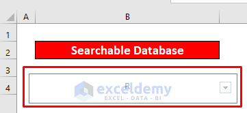
- Next, drag the mouse to properly resize the ComboBox as shown below.
- After that, you will see a new ComboBox created as follows.
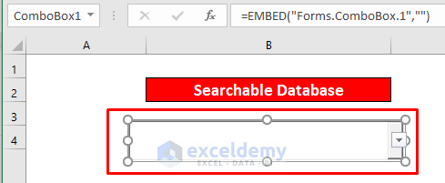
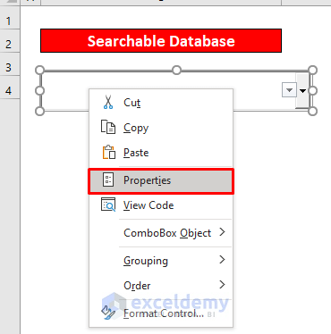
- Now right-click on the ComboBox and select Properties.
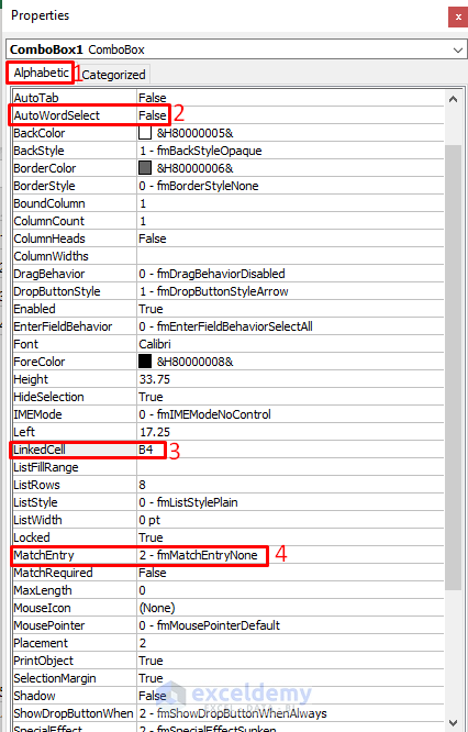
- After that, select the Alphabetic tab in the Properties window. Then make the following changes: AutoWordSelect >> False, Linked Cell >> B4, MatchEntry >> 2 – fnMatchEntryNone.
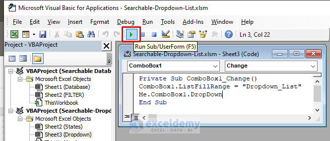
- Now copy the following code.
Private Sub ComboBox1_Change()
ComboBox1.ListFillRange = "Dropdown_List"
Me.ComboBox1.DropDown
End Sub- After that, double-click on the ComboBox. This will take you directly to a new module in the Microsoft VBA window. Then paste the copied code into the blank module as shown below. Then press F5 to run the code.
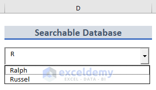
- Finally, the searchable database will work like Google Search.
Read More: How to Create a Simple Database in Excel VBA
Things to Remember
You can pop up the Microsoft Visual Basic for Applications window by pressing Alt + F11 simultaneously.
If a Developer tab is not visible in your ribbon, you can make it visible. To do that, go to,
File → Option → Customize Ribbon
You need to deselect the Design Mode in the Developer tab to be able to type in the ComboBox.
Download this practice workbook to exercise while you are reading this article.
Conclusion
I hope all of the suitable methods mentioned above to create a searchable dataset with VBA code will now provoke you to apply them in your Excel spreadsheets with more productivity. You are most welcome to feel free to comment if you have any questions or queries.
Related Articles
- How to Create a Database That Updates Automatically in Excel
- How to Create a Membership Database in Excel
- How to Create a Database in Excel with Pictures
<< Go Back To Database in Excel | Learn Excel
Get FREE Advanced Excel Exercises with Solutions!

