Troubleshooting Excel VLOOKUP Drag Down Issues (11 Solutions)

Dataset Overview

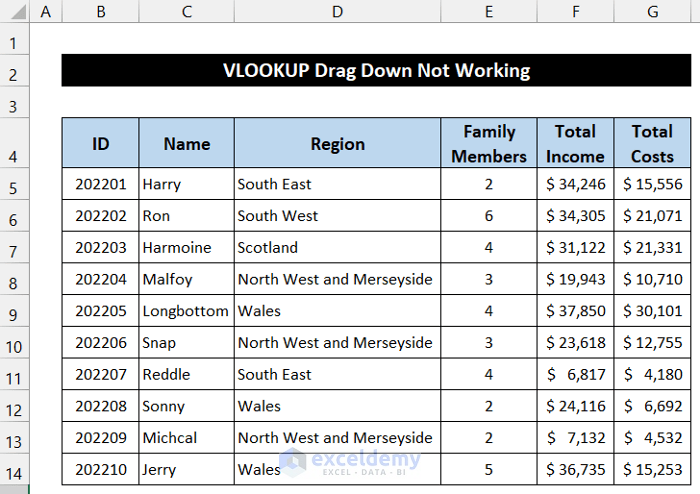
To demonstrate the solutions, we will use a dataset of 10 employees of any organization. The dataset contains employees’ IDs, names, residency areas, number of family members, incomes, and living costs. Our dataset is in the range of cells B5:G14.

The generic representation of the VLOOKUP function is given below:

Here,

• lookup_value: The value we are looking for keeping in the first column of our dataset or table.
• table_array: The table in which we look for the value.
• column_index_num: The column in the dataset or table from which we get our desired value.
• range_lookup: An optional requirement contains 2 cases, TRUE for the Approximate match, which is the default, and FALSE for the Exact match.

Solution 1 – Change Calculation Options

Sometimes Excel’s calculation settings can affect the accuracy of functions when dragging them down. To address this issue:

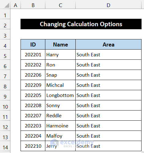
• Select any cell containing the VLOOKUP formula (e.g., D6).
• Check the formula in the Formula Bar.

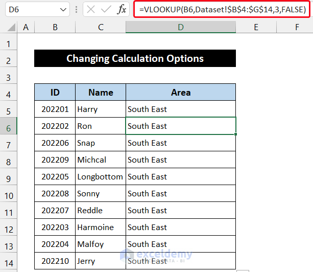
• If the result isn’t accurate, go to the Formula tab.
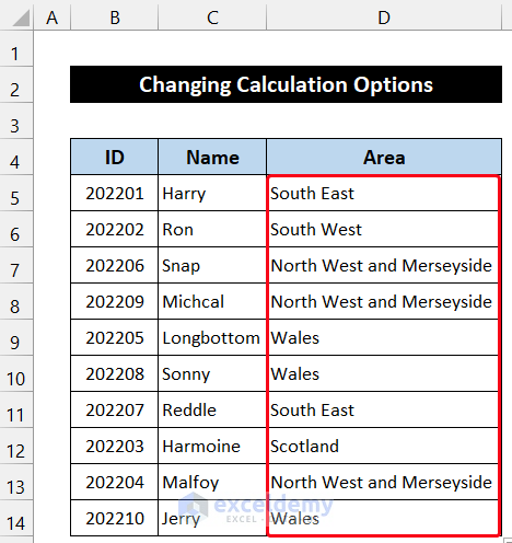
• Click the drop-down arrow next to Calculation Options and choose Automatic.

• The VLOOKUP function should now provide the correct result.

Solution 2 – Use Absolute Cell References in the Lookup Array

When writing the VLOOKUP function, ensure that the table_array reference contains absolute cell references. Otherwise, if the data’s position changes, the function may return incorrect results. Follow these steps:

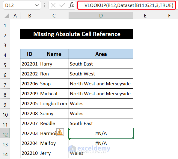
• Select cell D5 (where your VLOOKUP formula is).
• Confirm that the table_array reference includes the $ sign for absolute cell references.
• If not, modify the formula to include it, like this:

• Press Enter.

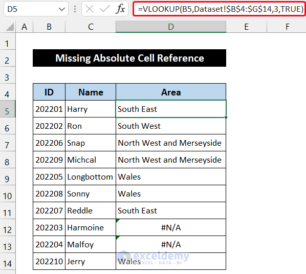
• Double-click the Fill Handle icon in cell D5 to copy the formula down to D14.
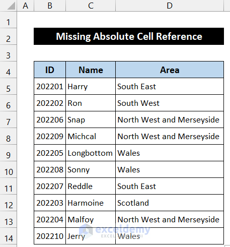
• The function should now return the correct values for the corresponding lookup values.

Solution 3 – Remove Duplicate Data from the Dataset

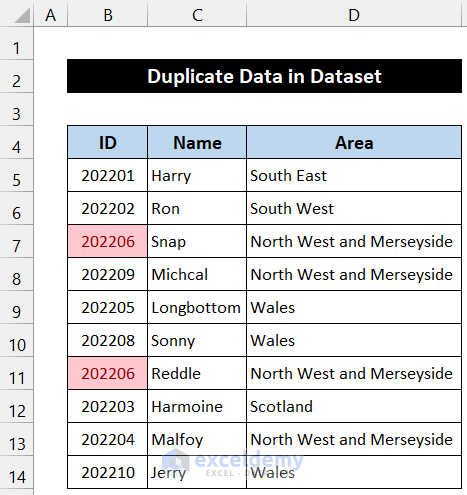
Duplicate data can wreak havoc when using VLOOKUP. Accidental double entries can lead to unexpected results. For instance, in our dataset, cell B11 doesn’t yield the expected South East value; instead, it shows North West and Merseyside.

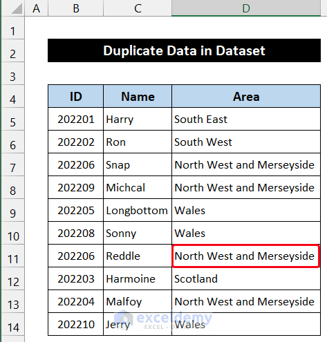
Here’s how to fix this:

• Select the range of cells B5:B14.
• In the Home tab, click the drop-down arrow next to Conditional Formatting in the Styles group.
• Choose Highlight Cell Rules and select Duplicate Values.

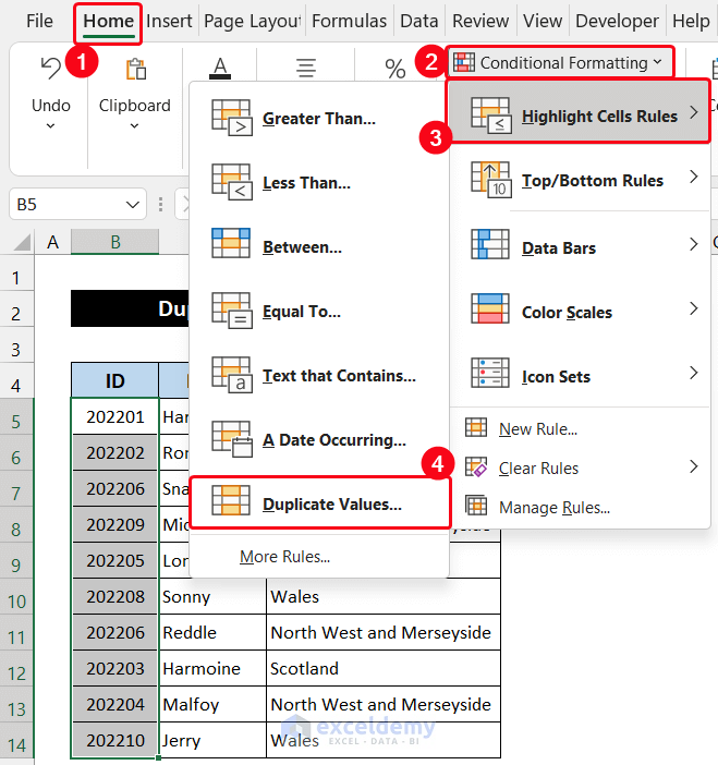
• You will see the duplicate values highlighted.

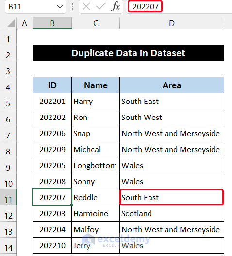
• Correct the duplicate value (e.g., enter the correct ID 202207).
• Cell D11 now displays the desired result.

Solution 4 – Keep Data Matching with Approximate Match

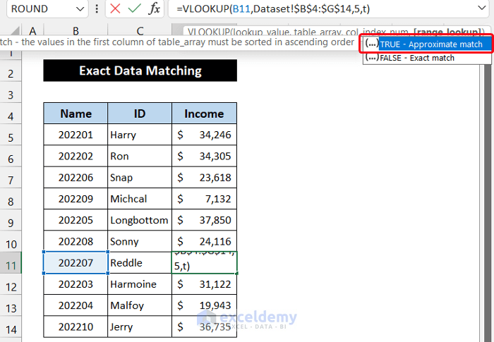
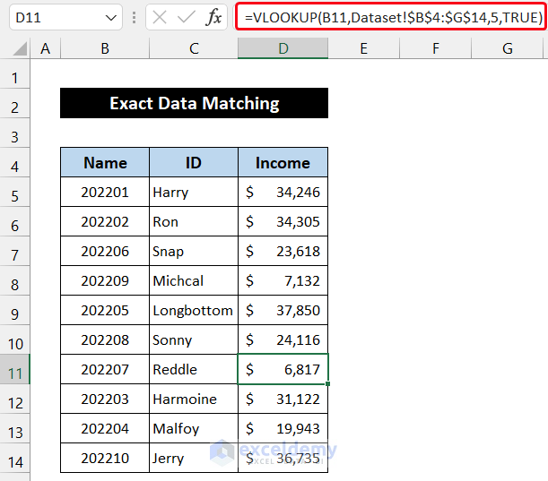
Exact data matching isn’t always necessary. In cell D11, we encounter a similar issue. To address it:

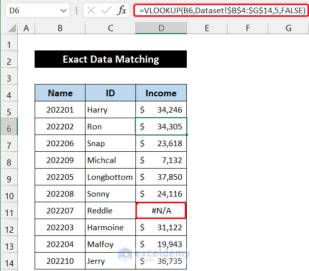
• Check the formula in cell D11.
• Change the match type from TRUE to FALSE:

• Press Enter.
• The function should now retrieve the value from the main dataset.

Read More: [Solved]: Excel VLOOKUP Not Working with Numbers

Solution 5 – Eliminate Empty Cells from the Dataset

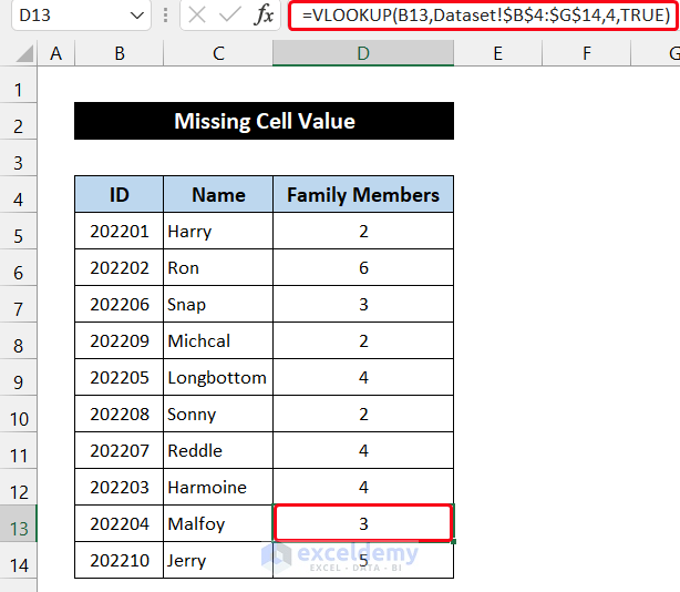
Accidentally deleting cell values disrupts Excel’s ability to extract data. In our dataset, cell D13 shows a problematic 0. Let’s fix it:

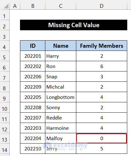
• Go to the main Dataset sheet.
• Manually enter the deleted cell value (you can select the data range).
• Press Enter.

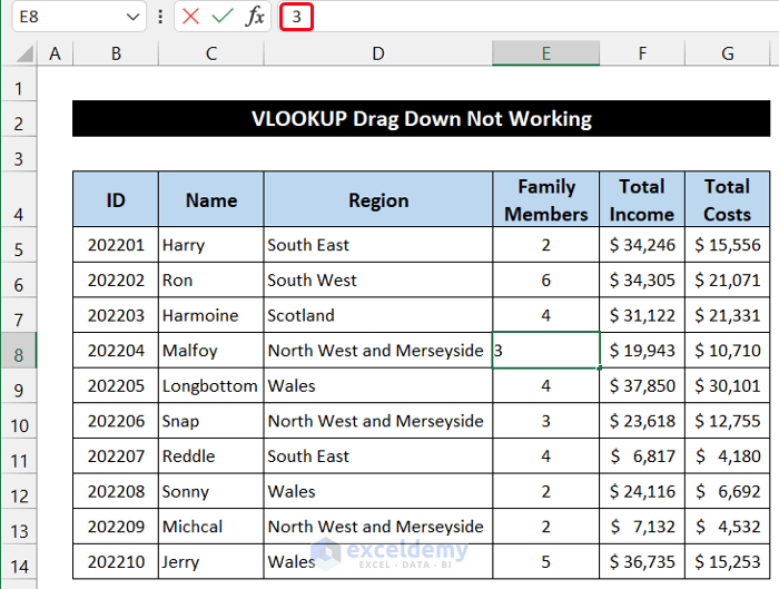
• Return to the previous sheet—the problem is resolved.

Solution 6 – Type Accurate Lookup Value

Incorrect lookup cell references can cause chaos. In our dataset, cells D5:D14 display a #N/A error due to this issue. Here’s the solution:

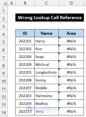
• Check cell D5’s function argument.

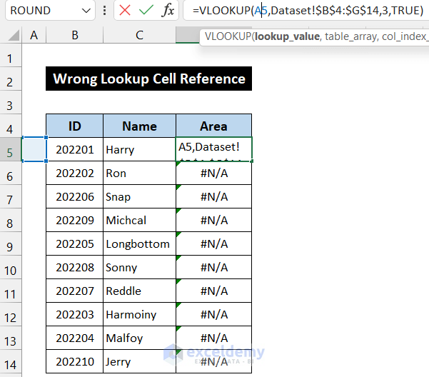
• Correct the reference from A5 to B5:

• Press Enter.

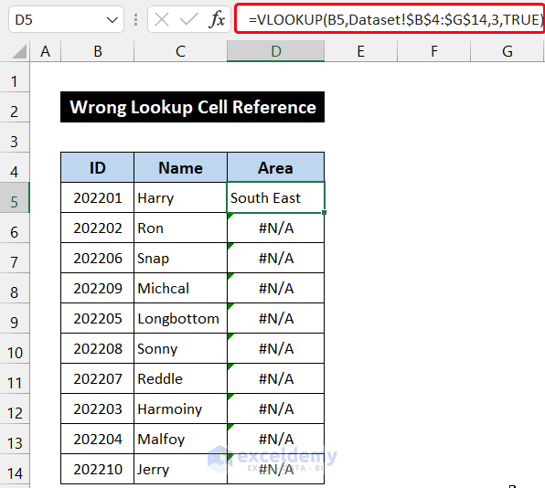
• Double-click the Fill Handle icon in cell D5 to copy the formula down to D14.

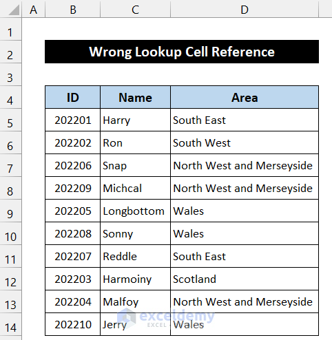
Solution 7 – Store Lookup Value in the Leftmost Column

The VLOOKUP function relies on the leftmost cell of our original dataset as the lookup_value. Failing to do so results in unexpected values, as shown in the image below. To fix this:

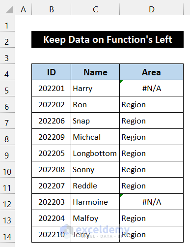
• Select cell D5.
• Modify the lookup_value cell reference from C5 to B5:

• Press Enter. The function will display the desired result.

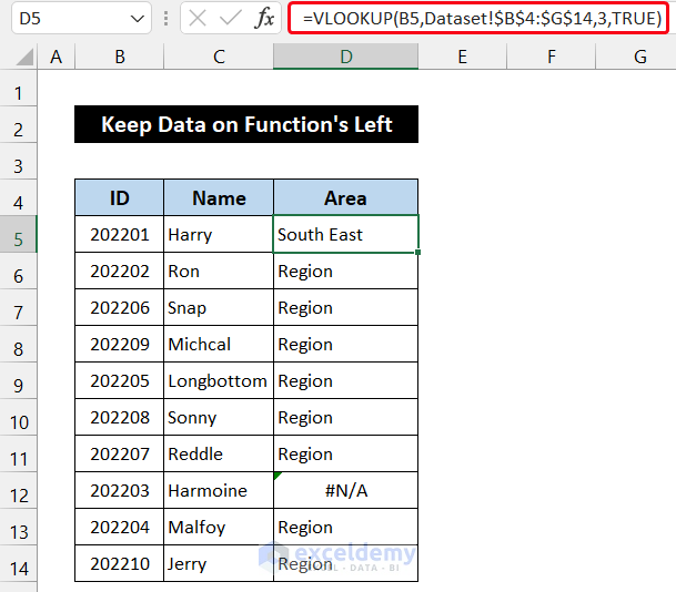
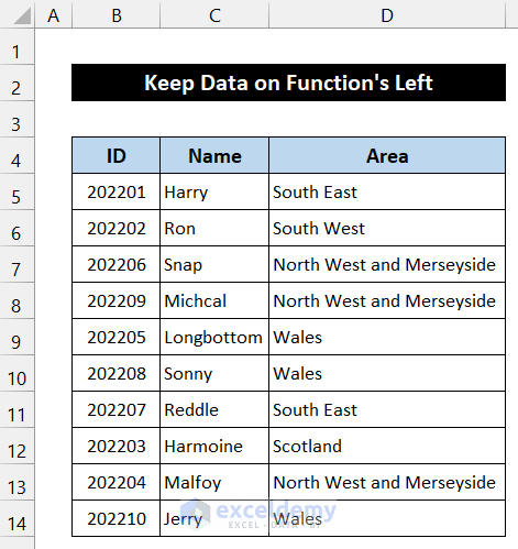
• Double-click the Fill Handle icon in cell D5 to copy the formula down to D14.
• The issue will be resolved, and you’ll obtain values for all employees.

Solution 8 – Insert Correct Column Index Number

Adding a new column can disrupt the VLOOKUP function, altering the column_index_num and preventing the desired results. In our dataset, all numbers turned to 0 due to this issue. Here’s the solution:

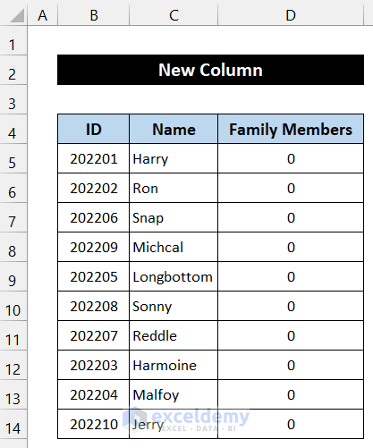
• Select cell D5 in the Formula Bar.
• Enter the correct column_index_num (in our case, 5):

• Press Enter.

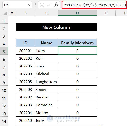
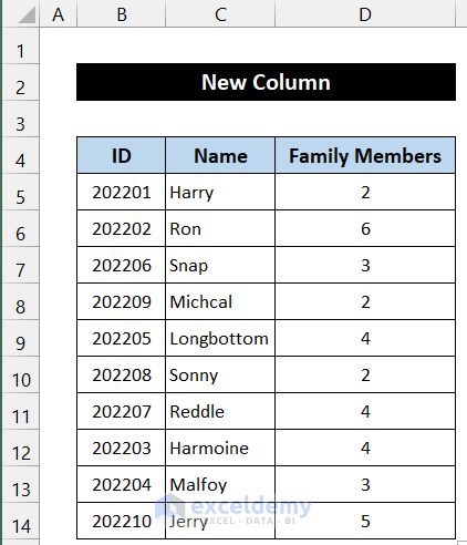
• Double-click the Fill Handle icon in cell D5 to copy the formula up to cell D14.
• The hitch will be resolved, and you will obtain value for all the entities.

Solution 9 – Choose Correct Table Array

Incorrect table_array references lead to #N/A errors in the dataset. If the VLOOKUP function encounters this issue, the drag down won’t work either. In our file, cells D5:D14 exhibit similar #N/A errors. Here’s how to fix it:

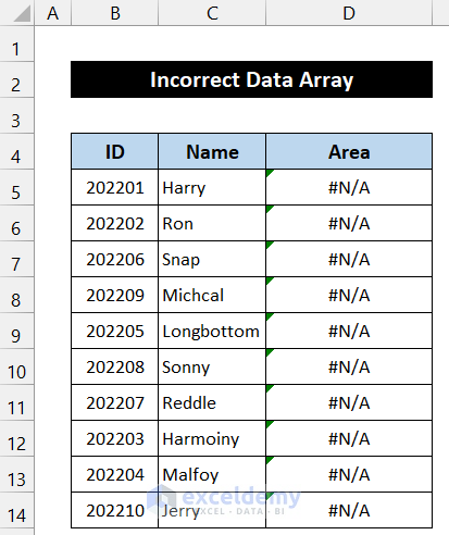
• Select cell D5 to check the function argument in the Formula Bar.
• Enter the proper function with an accurate table_array:

• Press Enter.

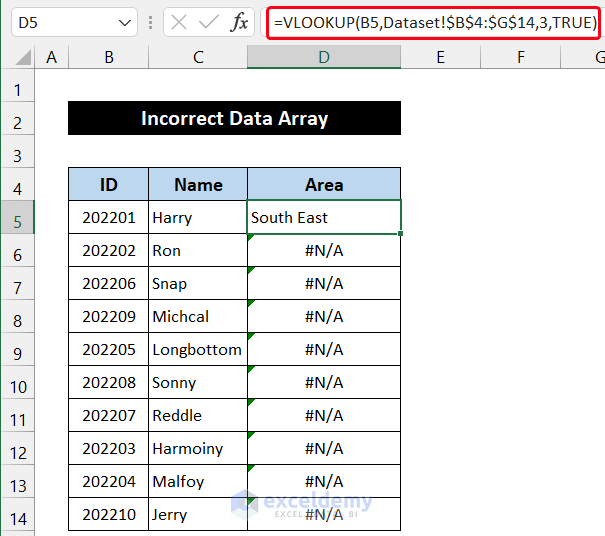
• Double-click the Fill Handle icon to copy the new formula up to cell D14.
• You’ll obtain all the desired values.

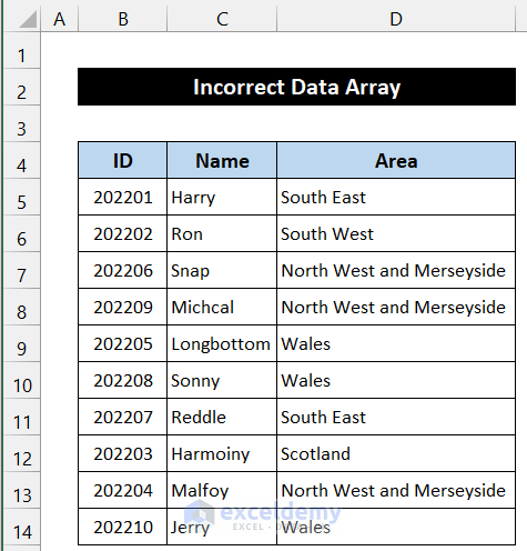
Solution 10 – Set Relevant Cell Format

Cell formatting can cause trouble when importing data from one sheet to another using the VLOOKUP function. Unpredictable values may appear due to incorrect cell formatting. Follow these steps:

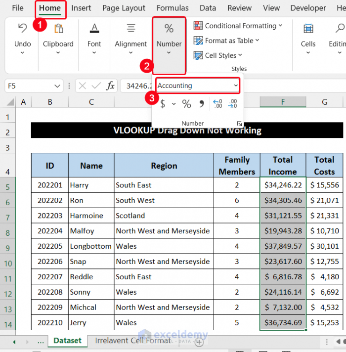
• Go to your original datasheet (in our file, it’s the Dataset sheet).
• Check the data format by selecting any cell in that column.
• Verify the data types from the Number group in the Home tab.

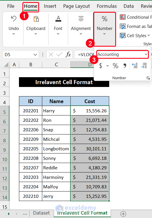
• Return to the sheet where you used the function (our workbook’s sheet titled Irrelevant Cell Format).
• Select the entire range of cells D5:D14.
• From the Number group in the Home tab, choose a similar data type (e.g., Accounting).
• The cell values will now match the original dataset.

Solution 11 – Remove Invisible Dash

Invisible dashes can cause errors with the VLOOKUP function. To fix this issue:

• Go to your original dataset and identify the entity causing the problem.
• Delete the existing data and manually enter it again.

The problem will be solved, and you will get your desired data.

Download Practice Workbook

You can download the practice workbook from here:

Related Articles

• [Fixed!] Excel VLOOKUP Not Working Due to Format
• [Fixed!] VLOOKUP Not Working Between Sheets
• VLOOKUP Not Picking up Table Array in Another Spreadsheet

<< Go Back to Issues with VLOOKUP | Excel VLOOKUP Function | Excel Functions | Learn Excel