Method 1 – Creating a Table to Refresh Chart in Excel
Step 1:
- Select the data range. From our dataset, we will select B4 to D10 for the convenience of our work. From your Insert tab, go to:
Insert → Tables → Table
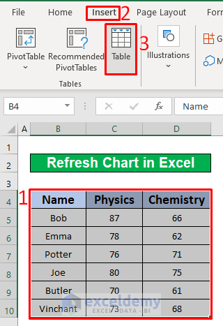
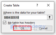
- Create Table dialog box will appear in front of you. From the Create Table dialog box, press OK.
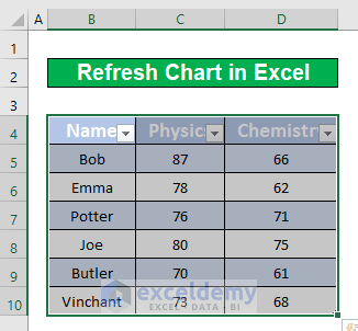
- Create a table which has been given in the below screenshot.
Step 2:
- Make a chart to refresh. To do that, firstly select the table range B4 to D10 from your Insert tab, go to:
Insert → Charts → 2-D Column
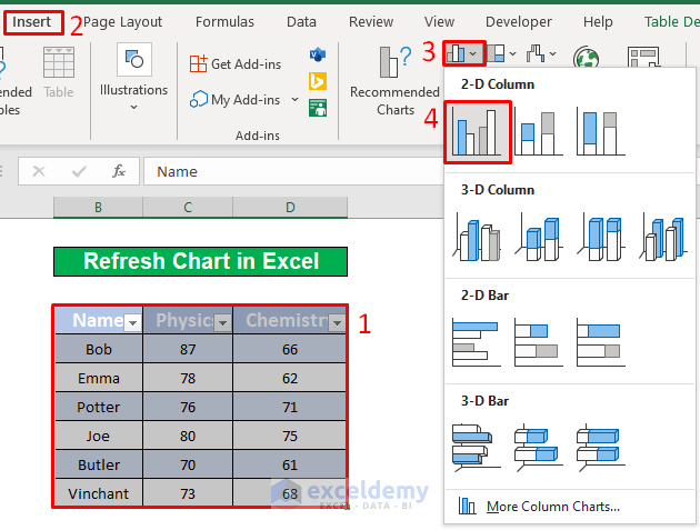
- You will be able to create a 2-D Column.
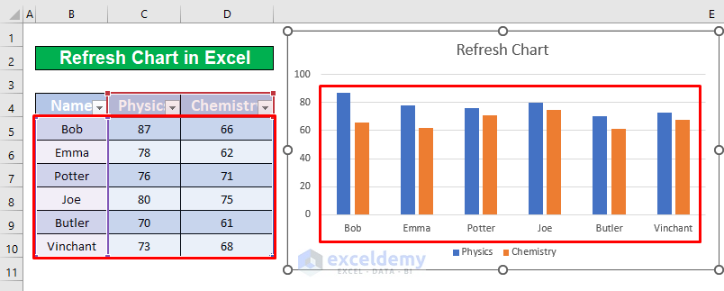
Step 3:
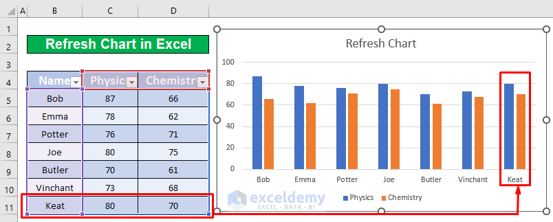
- Add a row to our table to refresh the chart. Keat’s securing marks in Physics and Chemistry are 80 and 70; we noticed that our chart will refresh automatically, as shown in the screenshot below.
Method 2 – Using Dynamic Formula to Refresh Chart in Excel
Step 1:
- Make the defined name and the dynamic formula for every column. From your Formulas tab, go to:
Formulas → Defined Names → Defined Name

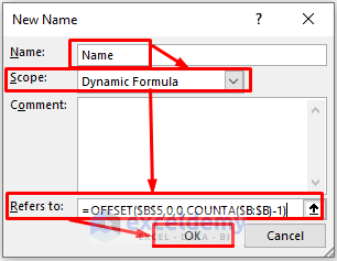
- A New Name dialog box will appear in front of you. From the New Name dialog box, type Name in the Name typing box. Select the current worksheet named Dynamic Formula from the Scope drop-down box. Type the below formulas in the Refers to typing box. The formulas are:
=OFFSET($B$5,0,0,COUNTA($B:$B)-1)- The OFFSET function indicates the first data and the COUNTA function indicates the entire column data.
- Press OK.
Step 2:
- Repeat Step 1 for columns C and D. The formula for the Physics column is:
=OFFSET($C$5,0,0,COUNTA($C:$C)-1)- The formula for the Chemistry column is,
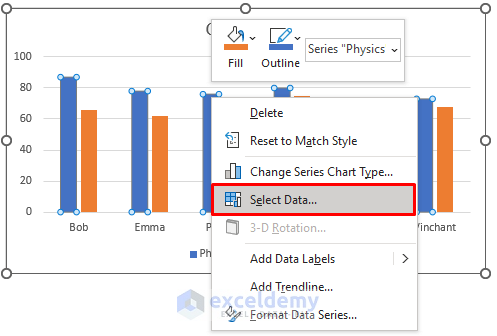
=OFFSET($D$5,0,0,COUNTA($D:$D)-1)- Press right-click on any column of your chart. A window pops up. From that window, select the Select Data option.
- A Select Data Source dialog box will appear in front of you. From the Select Data Source dialog box, select Physics. Select the Edit option under the Legend Entries (Series).
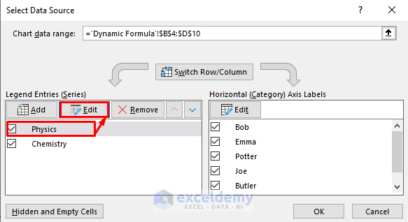
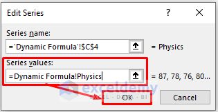
- A window named Edit Series pops up. From the Edit Series dialog box, type =’Dynamic Formula’!Physics in the Series values typing box. Press OK.
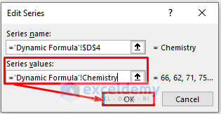
- From the Edit Series dialog box, type =’Dynamic Formula’!Chemistry in the Series values typing box. Press OK.
Step 3:
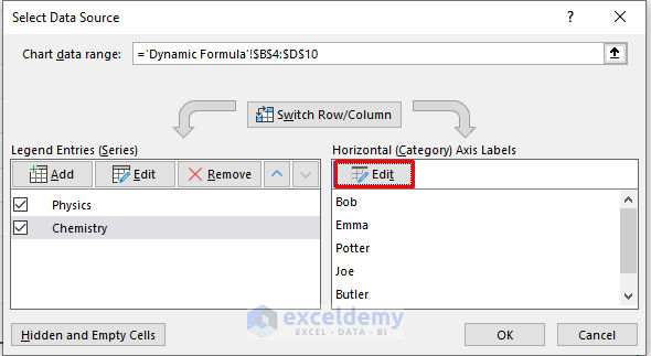
- Select the Edit button under the Horizontal (Category) Axis Labels option.
- An Axis Labels dialog box pops up. From the Axis Labels dialog box, type the below formula in the Axis label range typing box. The formula is:
='Dynamic Formula'!Name- Press OK.
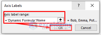
- Press OK.
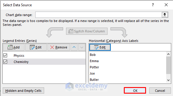
Step 4:
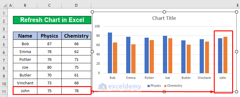
- Add a row to our table to refresh the chart. Add John’s securing marks in Physics and Chemistry to 75 and 78; we notice that our chart will refresh automatically, as given in the screenshot below.
Things to Remember
➜ While a value can not found in the referenced cell, the #N/A error happens in Excel.
➜ To create a table, you can press Ctrl + T simultaneously on your keyboard.
Download Practice Workbook
Download this practice workbook to exercise while you are reading this article.
<< Go Back To Excel Charts | Learn Excel
Get FREE Advanced Excel Exercises with Solutions!


If for some moments I have no data at all, I get error.
What can I do?
Hello BABA,
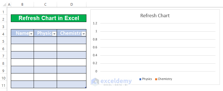
I have checked all of the methods of the above article again that can figure out how to refresh chart in excel. I think the article is appropriate to refresh chart in Excel. While removing data from the dataset, I would not get any error. Look at the below screenshot.
Thank you for your comment.
If you get error, please mail me personally at below mail address.
[email protected]
Regards
Md. Abdur Rahim Rasel (Exceldemy Team)