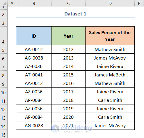
Let’s say we have a dataset that depicts the employee ID, the Year, and the Sales Person of the Year. We’ll use the dataset (in B4:D14 cells) shown below to count occurrences of names.
Method 1 – Using the COUNTIF Function to Count Exact Matches
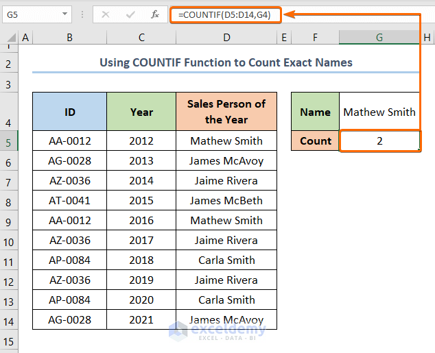
- We entered a name in the G4 cell.
- The formula in the G5 cell will be:
=COUNTIF(D5:D14,G4)The D5:D14 cells represent the Sales Person of the Year (range argument), and the G4 cell denotes Mathew Smith (criteria argument).
Formula Breakdown
- The COUNTIF function matches the name from cell F4 in the lookup array (D5:D14) and returns the number of counts.
Method 2 – Applying a Wildcard Character to Count Specific Names
Case 2.1 – If Cell Contains Specific Name at the Start
- We put the first name in the search cell G4.
- The formula in the G5 cell will be as follows.
=COUNTIF(D5:D14,G4&“*”)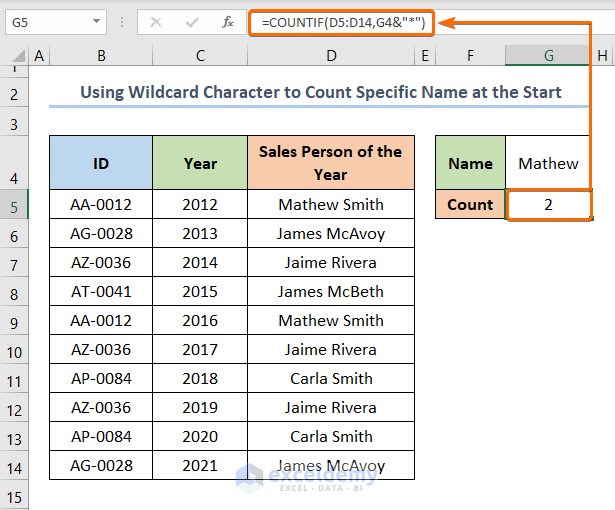
Case 2.2 – When the Name Is in the Middle
- The formula for the G5 cell will be as follows.
=COUNTIF(D5:D14,“*”&G4&“*”)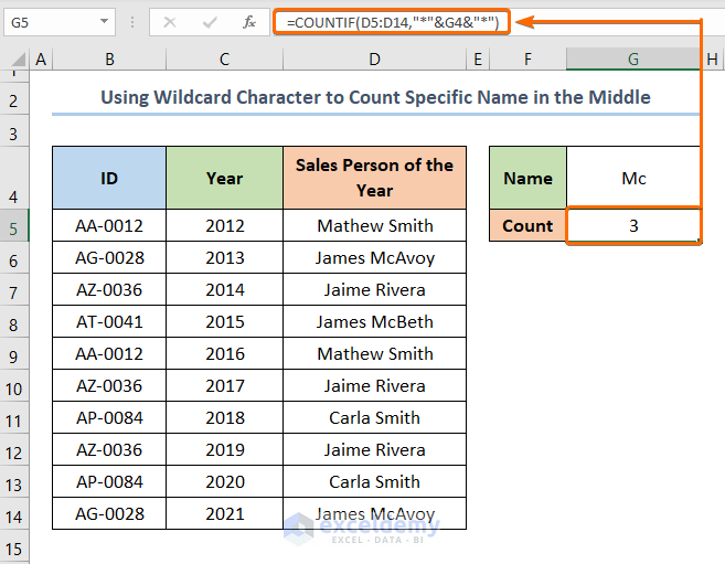
Case 2.3 – If the Name Is at the End
- The formula for the G5 cell will be as follows.
=COUNTIF(D5:D14,“*”&G4)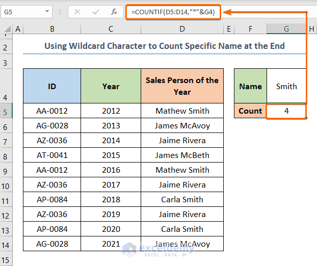
Method 3 – Utilizing the SUMPRODUCT Function to Count Specific Names in Excel
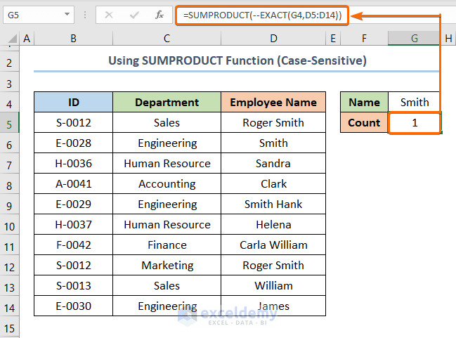
We have a table that shows the Employee ID, the Department they are employed in, and the Employee Name.

Case 3.1 – Applying the SUMPRODUCT Function to Match for the Exact Name (Case-Sensitive)
- Use the following formula:
=SUMPRODUCT(--EXACT(G4, D5:D14))The G4 cell denotes Smith (text1 argument) and the D5:D14 cells represent the Employee Name (text2 argument).
Formula Breakdown
- The EXACT function compares two strings of text and returns true if they are an exact match. The double minus operator changes the TRUE and FALSE values to numeric values 1 and 0.
- The SUMPRODUCT function returns the sum of all the 1’s in the corresponding range which represents the number of matches.
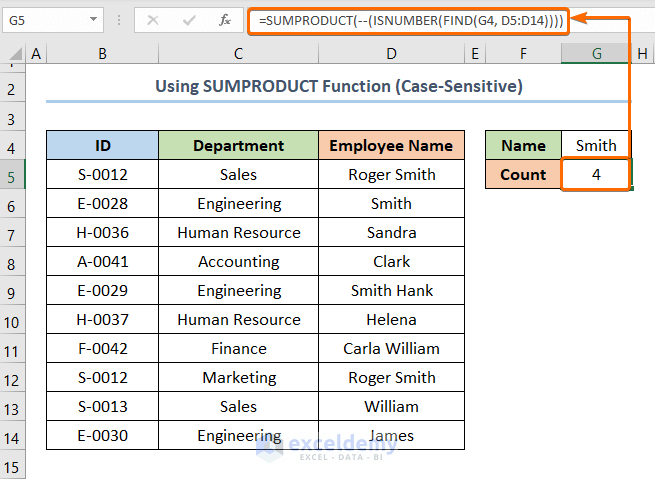
Case 3.2 – Using the SUMPRODUCT Function to Partially Match for a Name (Case-Sensitive)
- Use the following formula:
=SUMPRODUCT(--(ISNUMBER(FIND(G4, D5:D14))))The G4 cell denotes Smith (find_text argument) and the D5:D14 cells represent the Employee Name (within_text argument).
Formula Breakdown
- The FIND function gives the position (as numbers) of a text inside a string.
- The ISNUMBER function handles these numbers returned by the FIND function, which is then converted to 1 or 0 via the — operator.
- The SUMPRODUCT function adds up all the 1’s which represents the number of matches.
Case 3.3 – Using SUMPRODUCT Function to Count Names (Case-Insensitive)
- Use the following formula:
=SUMPRODUCT(--(ISNUMBER(SEARCH(G4, D5:D14,))))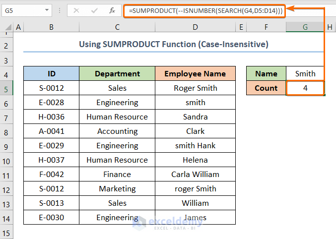
Formula Breakdown
- The SEARCH function determines the location (as number) of a text inside a string.
- The ISNUMBER function converts the numbers provided by the SEARCH function to ones and zeroes.
- The SUMPRODUCT function returns the number of counts.
Things to Remember
- The COUNTIF function returns integer output.
- The COUNTIF function does not count the cells with non-numeric values, like text or #NA.
- COUNTIF function is unable to count specific numbers within a number like “123” from “4546123”
- For columns with a mixture of text and numbers, the COUNTIF function gives the wrong count.
Download the Practice Workbook
<< Go Back to Count Words | Learn Excel
Get FREE Advanced Excel Exercises with Solutions!

