Common Salary Sheet Components
Part 1 – Employee Database and Salary Structure
This section contains a list of employees and their basic salaries, as well as all fixed modifiers that need to be applied to the salary to get the net earnings

Part 2 – Gross Salary Calculation
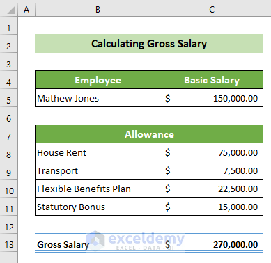
This section allows you to calculate the allowances for each employee. The allowances include the house rent allowance, transport allowance, and flexible benefits plan, and are listed in the Database section. The basic wage and the total allowances are summed up to calculate the gross salary:
Gross Salary = Basic Salary + Allowances
Part 3 – Calculation of Deductions
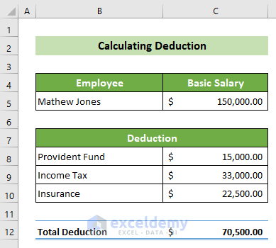
This section calculates deductions on the basic salary, per the information in the Database.
Part 4 – Net Payable Salary
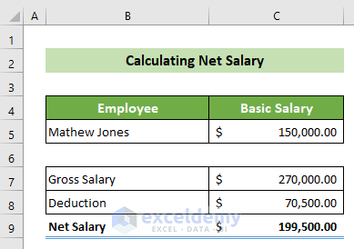
This section calculates the net payable salary:
Net Payable Salary = Gross Salary – Deductions
Make a Salary Sheet in Excel with Formula: Step-by-Step Procedure
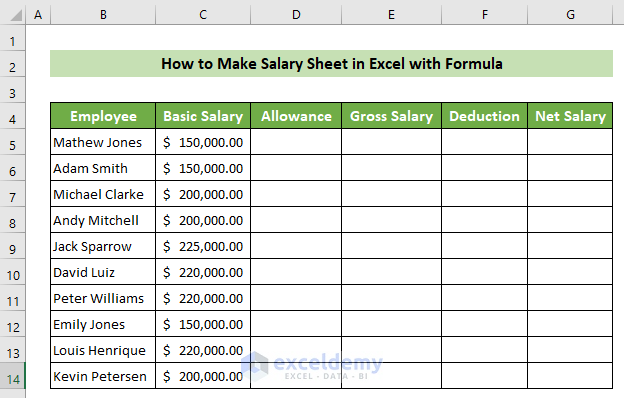
We have a dataset of a company with 10 employees.
Step 1 – Create the Employee Database and Salary Structure
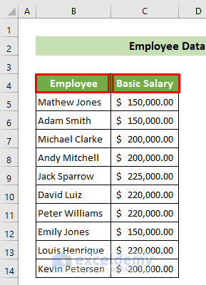
- Open a new worksheet and make two columns on the left side that will contain the employee names and their basic salaries.
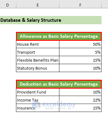
- Record the allowance percentages and deduction percentages of the company in a smaller dataset on the right.
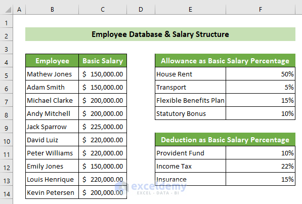
- Here’s our sample.
Step 2 – Calculate the Gross Salary
- Create a new sheet for the calculator.
- Click on the B5 cell.
- Go to the Data tab, select Data Validation (from Data Tools), and choose Data Validation….
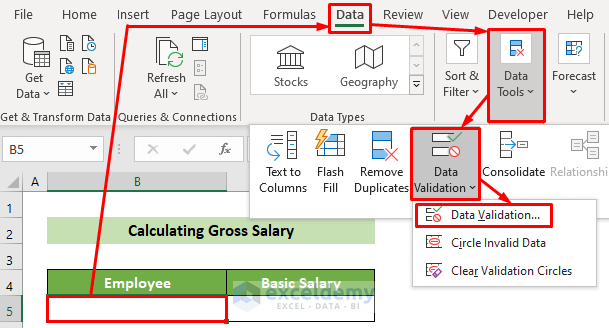
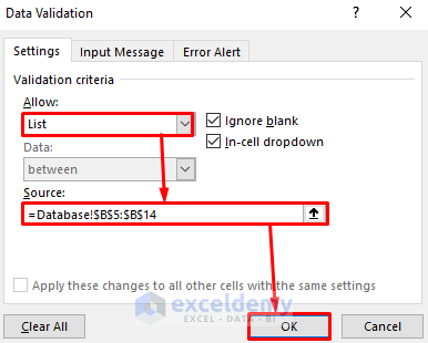
- The Data Validation window will appear. In the Settings tab, choose the option List from the Allow: drop-down list.
- In the Source: text box, refer to the cells B5:B14 of the Database worksheet.
- Click on the OK button.
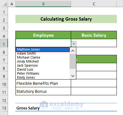
- The B5 cell has all the names of the employees in the dropdown list.
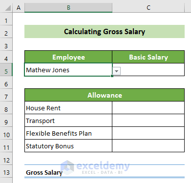
- We have chosen the first employee’s name.
- Select the C5 cell and insert the following formula, then press the Enter button.
=VLOOKUP(B5,Database!B4:C14,2,FALSE)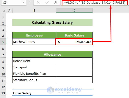
Formula Breakdown:
=VLOOKUP(B5,Database!B4:C14,2,FALSE)
It looks at the B5 cell value in the Database worksheet’s B14:C14 range. It returns the value that is in the same row as the found cell and in the second column of the array.
Result: 150,000
- Click on the C8 cell and insert the following formula, then press the Enter button.
=$C$5*VLOOKUP(B8,Database!$E$5:$F$8,2,FALSE)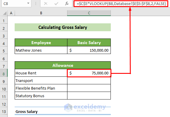
Formula Breakdown:
=VLOOKUP(B8,Database!$E$5:$F$8,2,FALSE)
It returns the value in the second column from the Database worksheet’s E5:F8 range where the value of the B8 cell from this worksheet is found there.
Result: 50%
=$C$5*VLOOKUP(B8,Database!$E$5:$F$8,2,FALSE)
Multiplies the C5 cell’s value with the previous result.
Result: $ 75,000
Note:
The data range (E5:F8) should be in absolute reference to avoid further errors when copying the formula. But, the lookup value (B8) should be in relative reference as it should be changed with respect to the allowance criteria. The basic salary (C5) reference should also be in absolute reference when multiplying. Use the dollar sign ($) or press the F4 key to make cell references absolute.
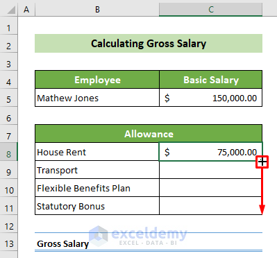
- Place your cursor in the bottom-right corner C8. A black fill handle will appear.
- Drag the fill handle down to copy the formula for all the allowances.
- To calculate the gross salary, click on the C13 cell and insert the following formula, then press the Enter button.
=SUM(C5,C8:C11) 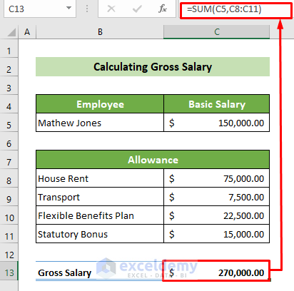
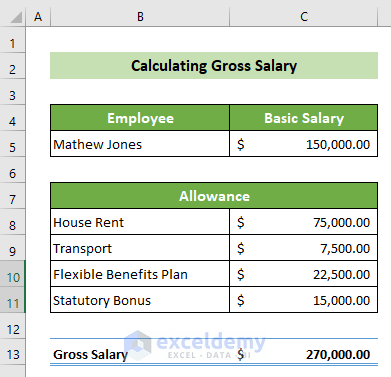
- Here’s our result.
Step 3 – Calculate Deductions
- Click on the B5 cell and refer to the Calculate Gross Salary sheet’s B5 cell.
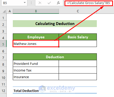
- Click on the C5 cell and refer to the Calculate Gross Salary sheet’s C5 cell.
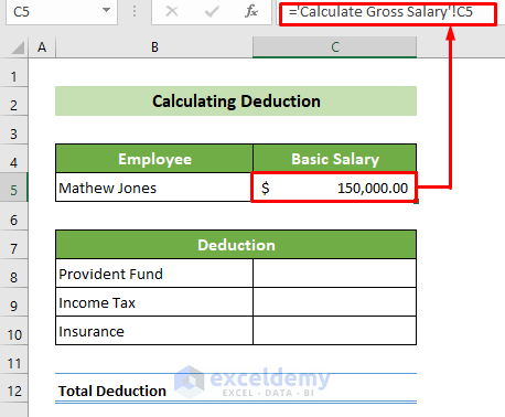
- Click on the C8 cell and use the following formula, then press the Enter button.
=$C$5*(VLOOKUP(B8,Database!$E$11:$F$13,2,FALSE))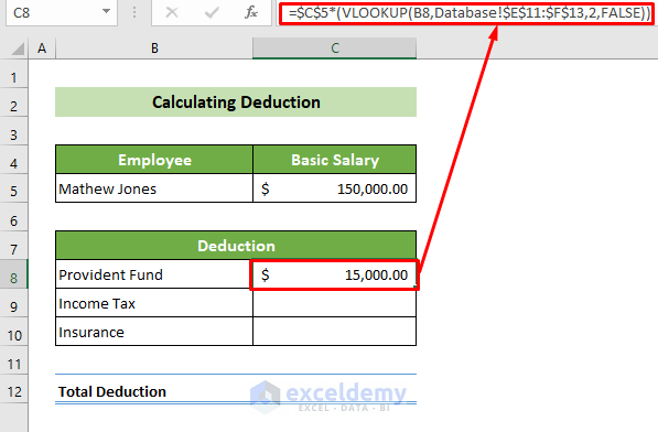
Formula Breakdown:
VLOOKUP(B8,Database!$E$11:$F$13,2,FALSE)
This returns the respective second column value from the Database worksheet’s E11:F13 range upon the condition of finding the B8 cell’s value from this worksheet in the specified range.
Result: 10%
=$C$5*(VLOOKUP(B8,Database!$E$11:$F$13,2,FALSE))
This multiplies the C5 cell’s value with the previous result.
Result: $ 15,000
Note:
The Database worksheet’s range (E11:F13) should be an absolute reference and the basic salary (C5) should also be an absolute reference when copying the formula. The lookup value (B8) should be in relative reference, as it changes with respect to your deduction criteria.
- Drag the fill handle down to fill the column.
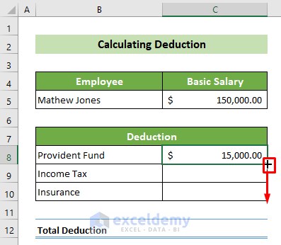
- Enter the following formula in C12:
=SUM(C8:C10)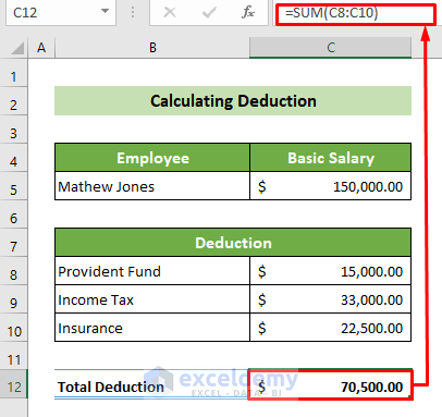
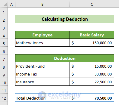
- Here’s our result.
Step 4 – Calculate the Net Salary
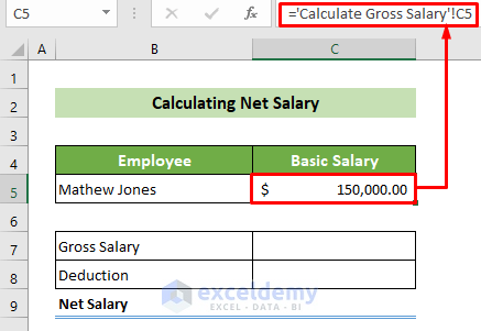
- Click on the C5 cell.
- Put an equal sign (=) and select cell C5 from the Calculate Gross Salary worksheet.
- Press the Enter button.
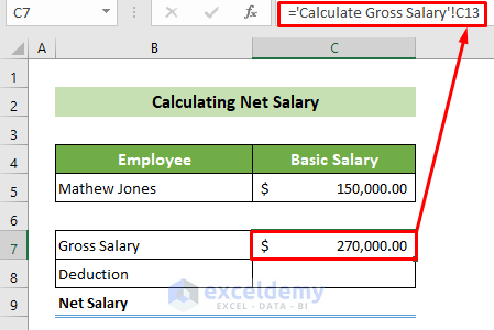
- Click on the C7 cell and link it with the C13 cell of the Calculate Gross Salary worksheet.
- Click on the C8 cell and link it with the Calculate Deduction worksheet’s C12 cell.
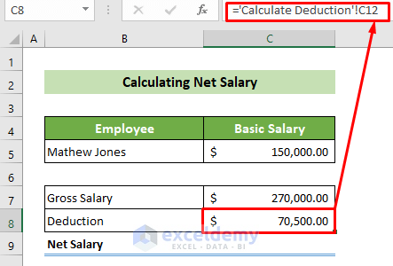
- Click on the C9 cell and insert the following formula, then press Enter.
=C7-C8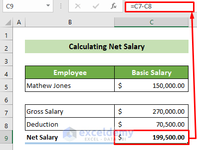
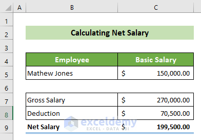
- Here’s the result.
Download the Sample Workbook
How to Make Salary Sheet in Excel: Knowledge Hub
<< Go Back to Salary | Formula List | Learn Excel
Get FREE Advanced Excel Exercises with Solutions!


IN OUT EXCLE SHEET MAIL SEND ME
Hi Abishek Sharma!
If you want the Excel file then you can download it from the Download Practice Workbook section. Or you need other assistance you can comment or send us mail at [email protected]
Great lesson, thank you very much
Dear OppaPanda,
You are most welcome.
Regards
ExcelDemy