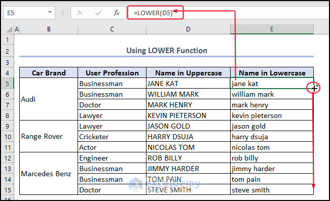
Change Upper Case to Lower Case in Excel: 6 Easy Methods

Method 1 – Applying LOWER Function

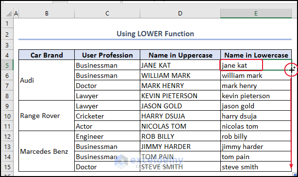
Type the following formula in cell E5.

=LOWER(D5)

Press ENTER.

Therefore, you will see the result in cell E5.

Drag down the formula with the Fill Handle tool.

You can see the complete Name in Lowercase column.

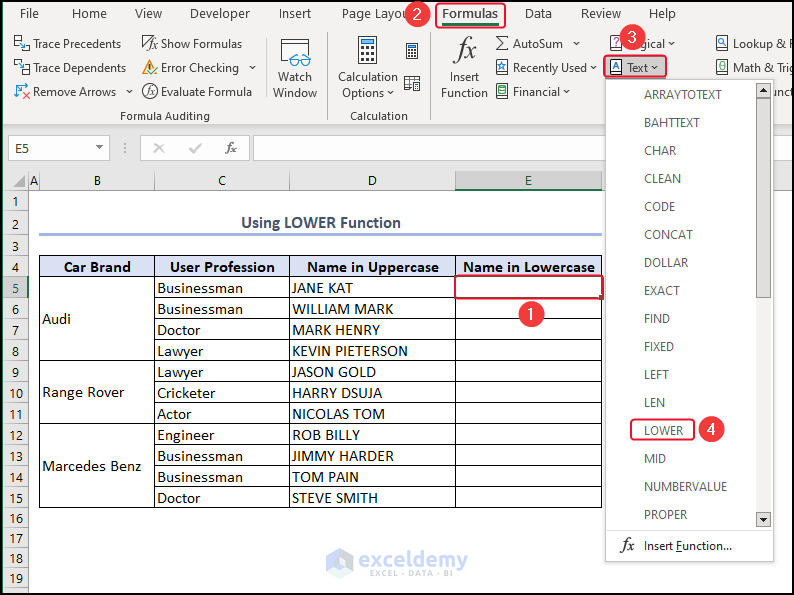
Inserting LOWER Function from Formula Tab

You can also insert the LOWER function from the Formula tab.

Click on cell E5 >> go to the Formulas
From the Text group >> click on LOWER.

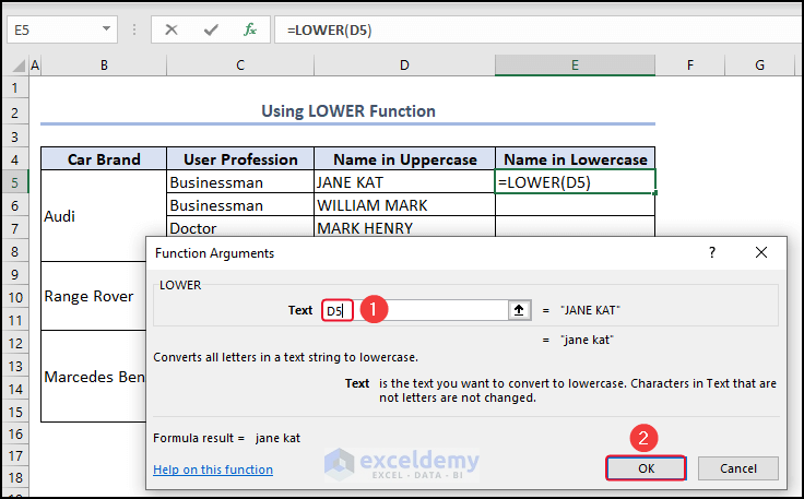
At this point, a Function Arguments dialog box appears.

Type D5 in the Text

Notice that cell E5 is showing the following formula.

=LOWER(D5)

Click OK.

See the output in cell E5.

Drag down the formula with the Fill Handle tool.

See the complete Name in Lowercase column.

Remove the Helper Column

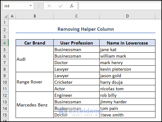
We have two name columns, one is the Name in Uppercase, which is the helper column. The other is Name in Lowecase. Once we have the complete Name in Lowercase column, we do not need the helper column anymore.

We will show how you can get rid of the helper column.

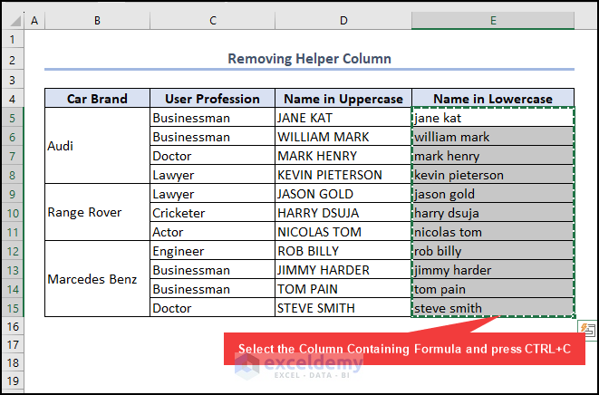
Select the column containing the formula, which is the Name in Lowercase
Press CTRL+C to copy this column.

Note: Remember to copy the column you want to stay in the dataset, not the helper column.

Copying a Column

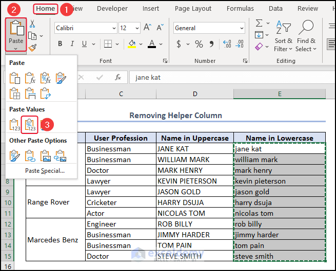
Go to the Home
From the Paste group > select the Paste Values

Select the helper column >> right-click on it.
Select the Delete option from the Context Menu.

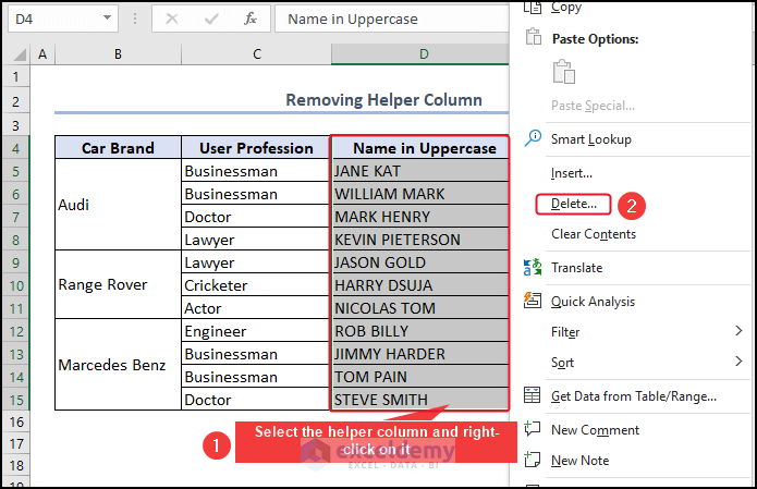
We removed the helper column and we have the columns that we need.

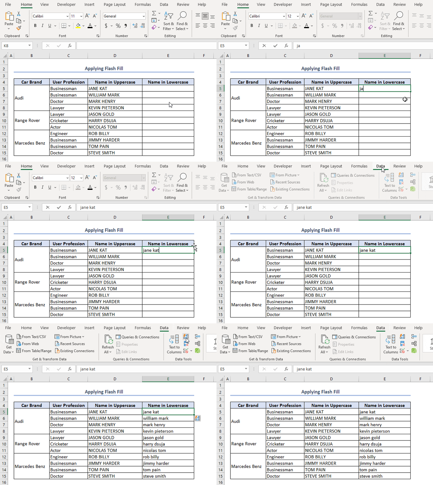
Method 2 – Use of Flash Fill Feature to Change Upper Case to Lower Case in Excel

Type the name of cell D5 in lowercase in cell E5.
Go to the Data
From the Data Tools group >> click on the Flash Fill

See all the cells contain names in lowercase.

Method 3 – Applying VBA to Change Upper Case to Lower Case in Excel

Go to the Developer tab >> select Visual Basic.

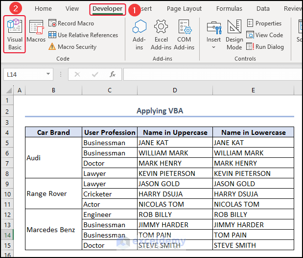
This will open a VBA Editor window.

Note: You can press the ALT+F11 keys to open the VBA Editor window.

From the Insert tab >> select Module.

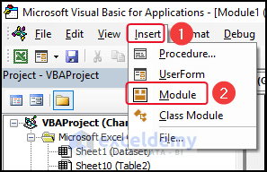
Type the following code in the Module.

Sub Change_Uppercase_to_Lowercase()
For Each i_cell In Selection
If Not i_cell.HasFormula Then
i_cell.Value = LCase(i_cell.Value)
End If
Next i_cell
End Sub
VBA Code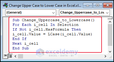

Code Breakdown

Sub Change_Uppercase_to_Lowercase()

We take Change_Uppercase_to_Lowercase as the Sub procedure.

For Each i_cell In Selection

We use For loop to run the loop through each selected i_cell.

If Not i_cell.HasFormula Then

We use the If statement to check whether i_cell contains a formula.

i_cell.Value = LCase(i_cell.Value)

End If

When the value of i_cell will equal the value of LCase i_cell, then the If statement will exit.

Next i_cell

This line ends the For loop.

End Sub

This line ends the Sub procedure.

Save the code >> return to our Worksheet.
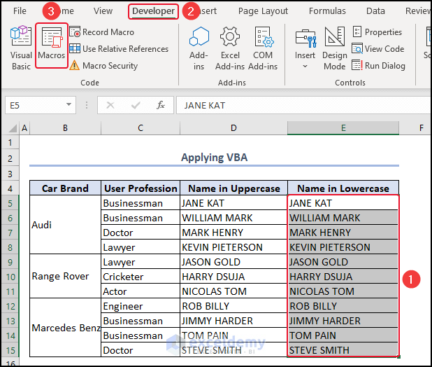
Run the code; we will select the Name in Lowercase columns >> go to the Developer tab >> select Macros.

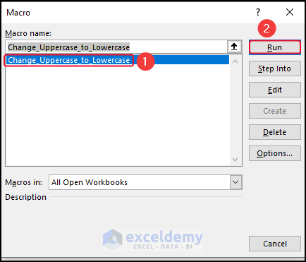
A Macros window will appear.

Select the Sub procedure >> click on Run.

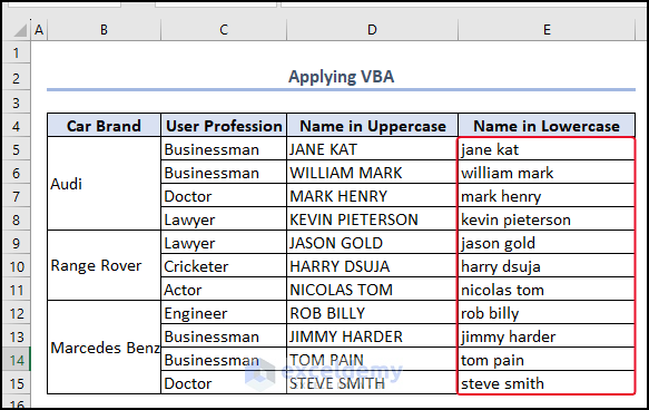
You can see the selected column now has names in lowercase.

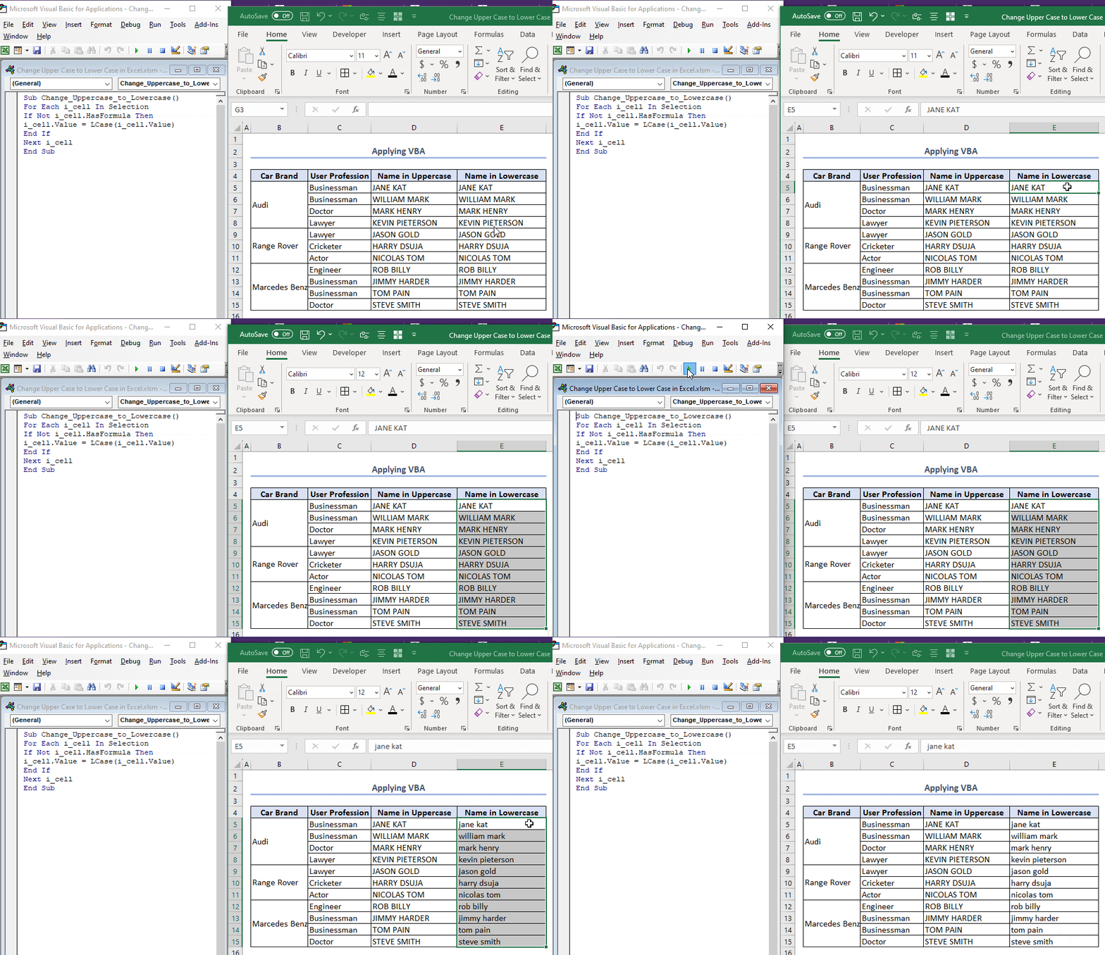
Check out the following GIF for a better understanding.

Method 4 – Using Microsoft Word

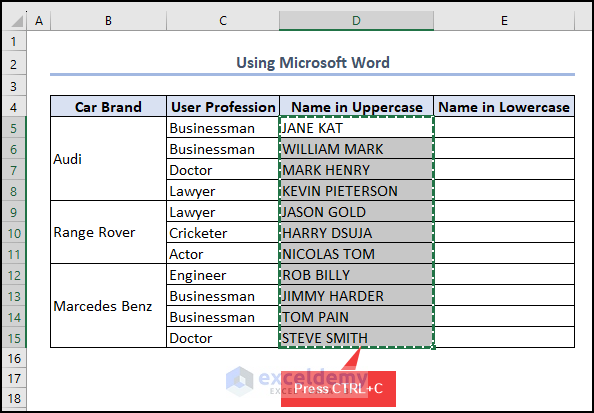
Select the Name in Uppercase column excluding the column header.
Press CTRL+C to copy.

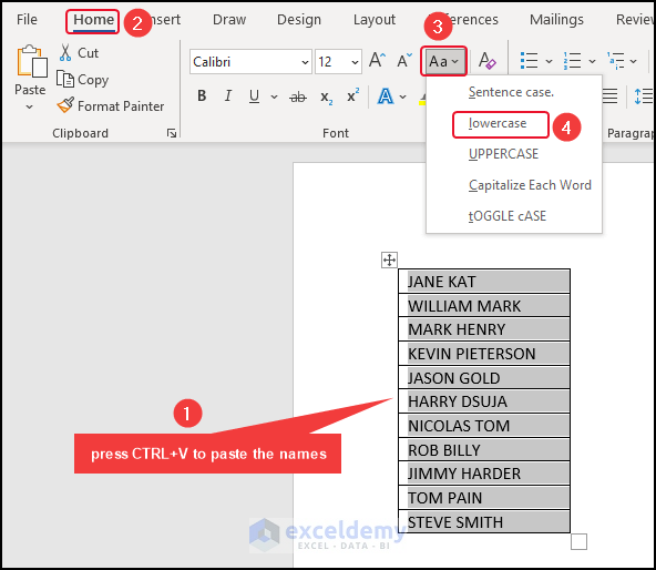
Open Microsoft Word, and paste the copied cells by pressing CTRL+V.
Go to the Home tab >> select the Change Case (Aa) icon >> select Lowercase.

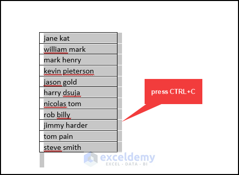
You can see the column has names in lowercase.

Copy these names by pressing CTRL+C.

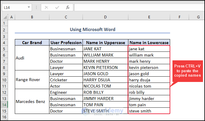
Go to the Excel sheet >> select the cells where you want to input the copied cells >> press CTRL+V to paste.

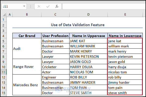
Method 5 – Use of Data Validation to Enter Text in Lower Case Only

Select cells E5:E15 >> go to the Data
From the Data Validation group >> select Data Validation.

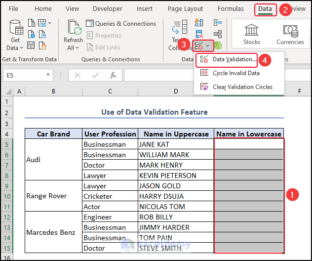
A Data Validation dialog box will appear.

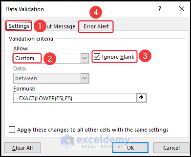
From Settings >> select Custom.
Mark the ignore blank box >> click on Error Alert.

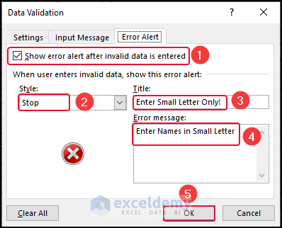
In the Error Alert window, mark Show error alert after invalid data is entered.

Select Stop as Style.
Type a Title >> type an Error message.
Click OK.

Try to type anything in uppercase; an error will pop up.

Click on Cancel >> type the name in lowercase.

At this point, no error message will pop up.

Press ENTER.

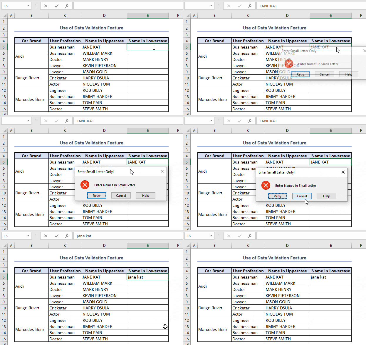
We completed the Name in Lowercase column by typing the name in lowercase.

Method 6 – Using Power Query to Change Upper Case to Lower Case in Excel

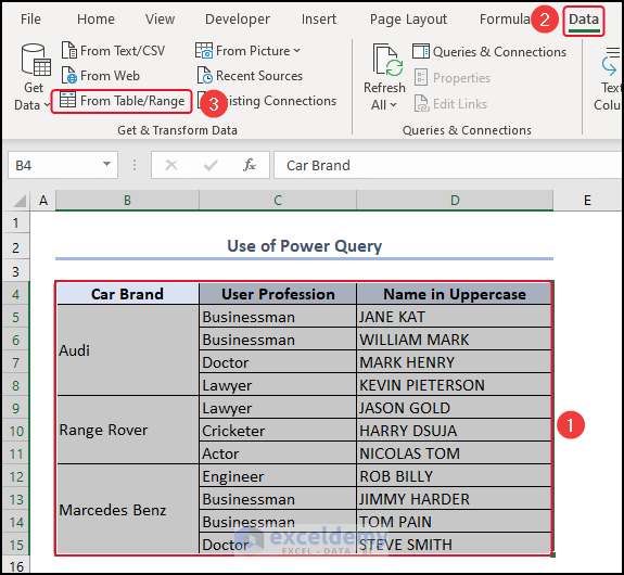
Insert Power Query, we will select the entire dataset >> go to the Data
From the Get & Transform Data group >> select From Table/Range.

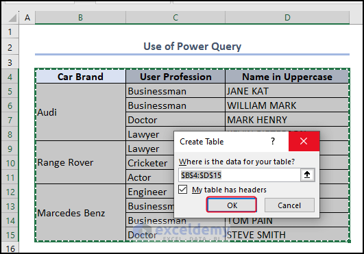
A Create Table dialog box will appear.

Make sure the My table has headers checkbox is marked >> click OK.

See the Power Query.

Select the Name in Uppercase column >> go to the Add Column
From the Format group >> select Lowercase.

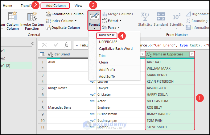
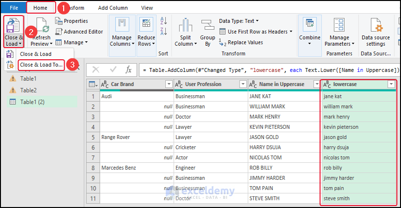
See a lowercase column.

Go to the Home tab >> click on Close & Load To.

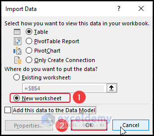
An Import Data dialog box will appear.

Select New Worksheet >> click OK.

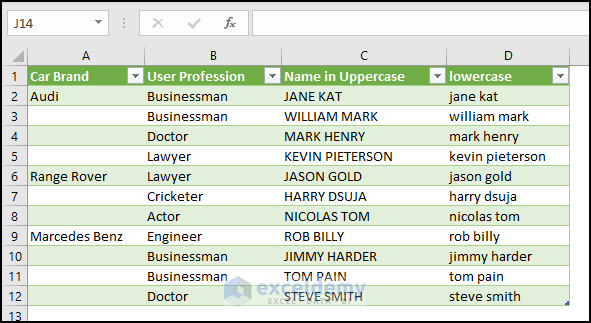
See the dataset having the lowercase column.

Things to Remember

Using the LOWER function is simple and easy among other methods to change uppercase into lowercase.
You can use Flash Fill by pressing ALT + E In many cases this doesn’t work. Then you can use the procedure that we have described above.
Power Query is a very effective tool in Excel not only to change text patterns but also to organize data in various ways.

Download Practice Workbook

You can download the Excel file from the link below and practice the explained methods.

Change Upper Case to Lower Case.xlsm