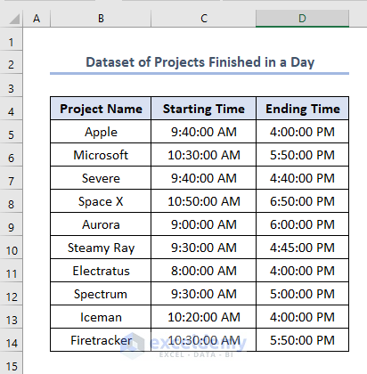
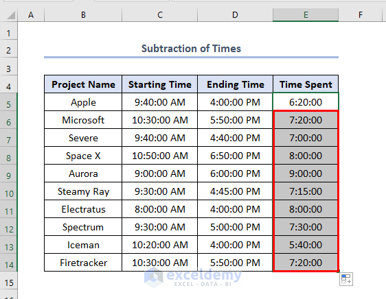
We have made a dataset named Dataset of Projects Finished in a Day. It has column headers as Project Name, Starting Time, and Ending Time. We’ll first consider that these projects end within a day. The dataset is like this.
Method 1 – Subtracting Two Times to Track Time Spent on Projects in Excel
- Use the following Subtraction formula in cell E5.
=D5-C5D5 is the Ending Time and C5 is the Starting Time of project Apple.
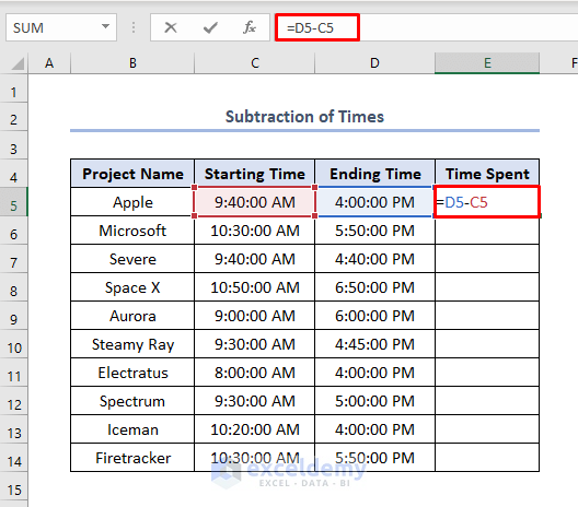
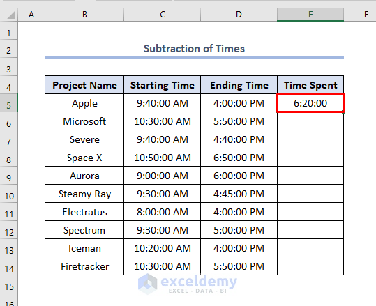
- Press Enter.
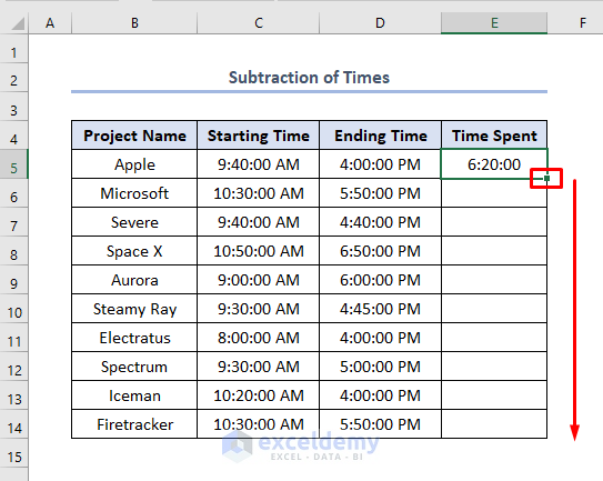
- Use the Fill Handle tool by dragging down the bottom-right corner of the reference cell E5.
We’ll get all the outputs from cell E6 to E14 like this.
Method 2 – Using the TEXT Function to Track Elapsed Time
We can get the output in a day or hour by using dd or hh text inside the formula.
- In the E5 cell, we can use the following formula for hour values.
=TEXT(D5-C5,”hh”)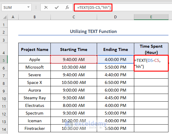
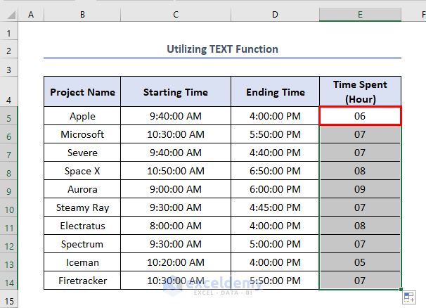
- Press Enter and use the Fill Handle to get the other outputs.
Method 3 – Applying the NOW Function to Calculate Elapsed Time Spent on Projects
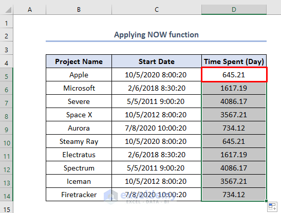
We know the Starting Time of a few ongoing projects.
- Insert the following formula in the D5 cell.
=NOW()-C5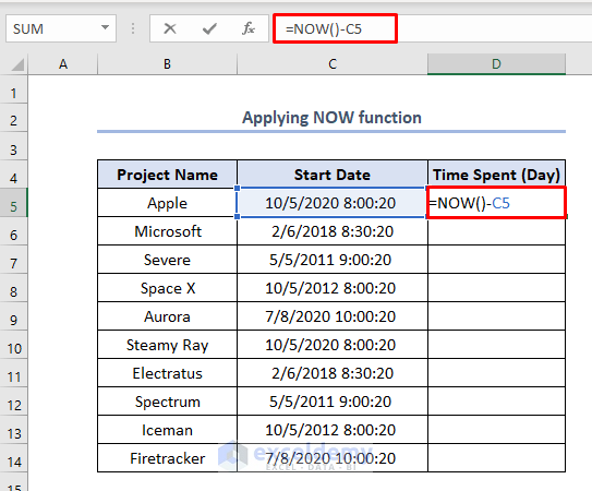
- Hit Enter and drag down the Fill Handle.
Method 4 – Using the TIME Function to Calculate the Time Spent
- Use the following function in D5:
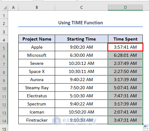
=TIME(HOUR(NOW()), MINUTE(NOW()), SECOND(NOW())) - C5Here, the NOW function will give the current time, then the HOUR, MINUTE, and SECOND functions will extract the hour, minute, and second portion of this time. Finally, the TIME function will return the result as a time. Eventually, the result will be subtracted from the value of C5.
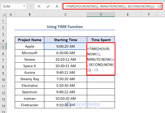
- Press Enter and use the Fill Handle to get all the outputs.
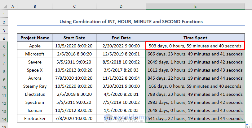
Method 5 – Applying Combinations of Functions to Show the Complete Time Difference
- We have the values in C and D columns and want to get the complete difference.
- Use this formula in the E5 cell:
=INT(D5-C5) & " days, " & HOUR(D5-C5) & " hours, " & MINUTE(D5-C5) & " minutes and " & SECOND(D5-C5) & " seconds"Formula Breakdown
- D5-C5 → returns the difference between the times in the cells D5 and C5.
- Output → 0414
- INT(D5-C5) → becomes
- INT(503.0414) →The INT function returns the integer value
- Output → 503
- INT(D5-C5) & ” days, ” → becomes
- 503 & ” days, ” → The Ampersand operator joins 503 with days.
- Output → 503 days,
- HOUR(D5-C5) → becomes
- HOUR(0.0414) →The HOUR function returns the value in hours
- Output → 0
- HOUR(D5-C5) & ” hours, ” → becomes
- 0 & ” hours, ” → The Ampersand operator joins 0 with hours.
- Output → 0 hours,
- MINUTE(D5-C5) → becomes
- MINUTE(0.0414) →The MINUTE function returns the value in minutes
- Output → 59
- MINUTE(D5-C5) & ” minutes and ” → becomes
- 59 & ” minutes and ” → The Ampersand operator joins 0 with minutes
- Output → 59 minutes and
- SECOND(D5-C5) → becomes
- SECOND(0.667) →The SECOND function returns the value in seconds
- Output → 40
- SECOND(D5-C5) & ” seconds ” → becomes
- 40 & ” seconds” → The Ampersand operator joins 0 with seconds
- Output → 40 seconds
- INT(D5-C5) & ” days, ” & HOUR(D5-C5) & ” hours, ” & MINUTE(D5-C5) & ” minutes and ” & SECOND(D5-C5) & ” seconds” → becomes
- 503 days, & 0 hours, & 59 minutes and & 40 seconds → The Ampersand operator joins the texts.
- Output → 503 days, 0 hours, 59 minutes and 40 seconds
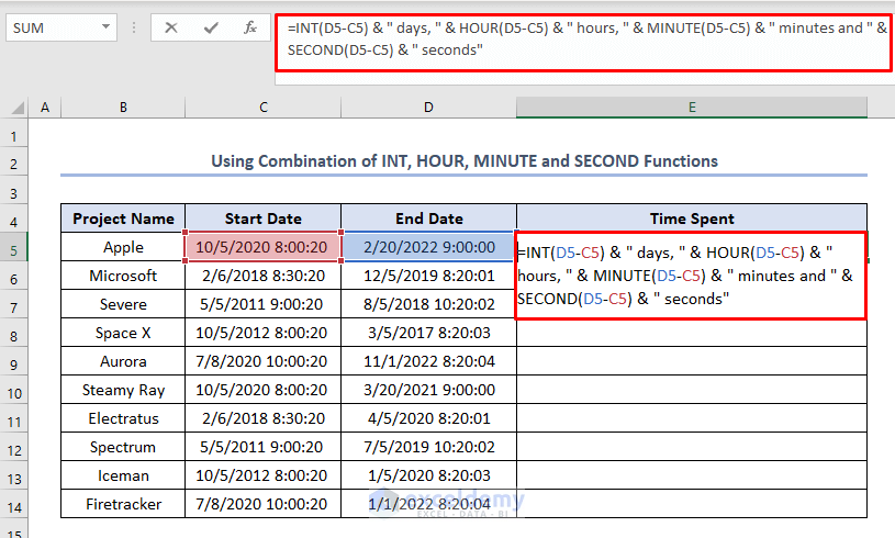
- Press Enter and use the Fill Handle to find all the outputs.
Download the Practice Workbook
Related Articles
- How to Track Project Progress in Excel
- How to Track Multiple Projects in Excel
- How to Create Project Pipeline in Excel


