How to Create Pay off Credit Card Debt Calculator in Excel

Pay off credit debt calculator is an essential staff for any person to check the amount of loan on his/her credit card. Using Microsoft Excel, you can easily design your credit card debt calculator. In this article, we are going to show you the step-by-step procedure of creating a pay-off credit card debt calculator in Excel. If you are also interested in designing your calculator, download our free template and follow us.

We are going to describe the step-by-step procedure to design a pay-off credit card debt calculator in Excel. After completing all the steps, the calculator will be like the image shown below:

Step 1: Designing the Preliminary Layout of the Credit Card Debt Calculator

In the first step, we will design the essential information area of the calculator.

First of all, the range of cells B2:F2.
Now, in the Home tab, click on the Merge & Center option from the group Alignment.

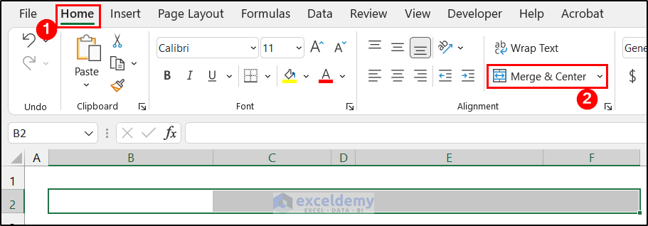
Then, write down a suitable title for this sheet according to your desire. We write down Credit Card Payoff Calculator for our sheet.

After that, in the range of cells B4:B7, write down the following entities and keep the corresponding cells for inputting the values.

Finally, we want to insert a data validation drop-down for the Card Type.
For that, select cell C7, in the Data tab, and click the drop-down of the Data Validation > Data Validation option from the group Data Tools.

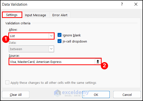
As a result, the Data Validation dialog box will appear.
In the Settings tab, change the Allow field from Any value to List and write down the following entities Visa, MasterCard, American Express in the Source field.
At last, click OK.

You will see a data validation drop-down will be added in that cell.

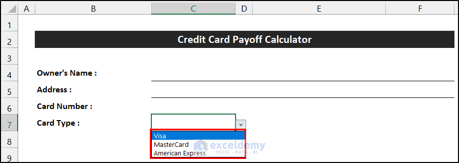
Our first task is finished here.

Thus, we can say that we have completed the first step to design a pay-off credit card debt calculator in Excel.

Step 2: Creating a Credit Card Information Section in the Debt Calculator

In this following step, we are going to create a section entitled Credit Card Information, where we have to input some important information about the credit card.

First, we will add the title of the section in the merged cell B9.

Then, write down the following entities in the range of cells B10:B12. Among them, we have to manually input the amount of the Current Balance and the Annual Interest Rate.

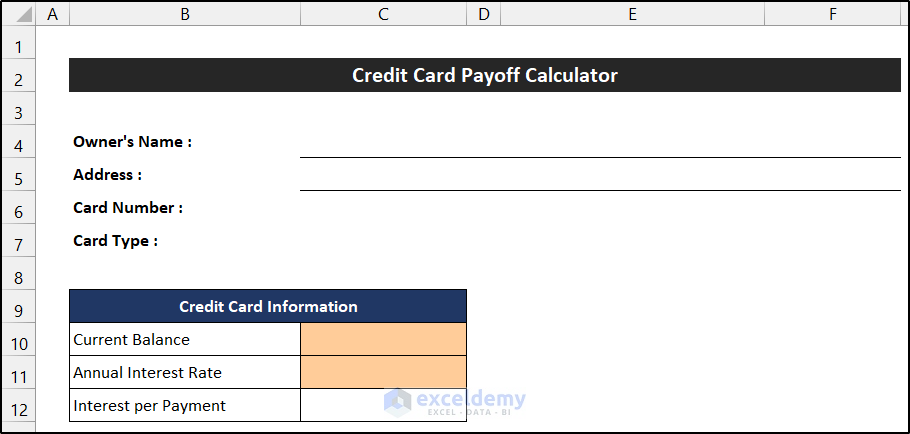
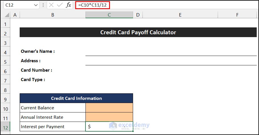
After that, write down the following formula to estimate the Interest per Payment in cell C12.

=C10*C11/12

Press Enter.

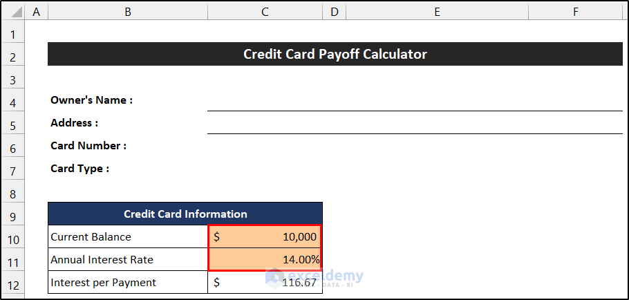
Let’s input some sample data in the range of cells C10:C11 to check the accuracy of our formula. We consider $10,000 as the Current Balance and the annual rate of interest as 14%.
You will get the value of the interest in cell D12.

Our job is completed.

So, we can say that we have finished the second step of designing a pay-off credit card debt calculator in Excel.

Step 3: Making User Input Section for the Credit Card Debt Calculator in Excel

Similarly, we will create the User Input section. In this section, the user of this calculator will input the value according to his/her desire.

Firstly, write the title of this section, User Input, like the previous section, in the merged cell E9.
Now, write down the following entities in the range of cells E10:E11, and format the corresponding cells to input the value at those cells.

The task of this section is completed.

Hence, we can say that we have accomplished the third step of creating a pay-off credit card debt calculator in Excel.

Step 4: Estimate Number of Months to Payoff Pay Credit Card Debt

Now, we are going to create a section where we will get the required number of months for any specific amount. To get the result from this section, we have to input the amount of money we are eligible to pay each month in cell F10.

Like the previous step, first, write down the title of this section in the merged cell B14.

Then, entitle the following entities in the range of cells B15:B17.

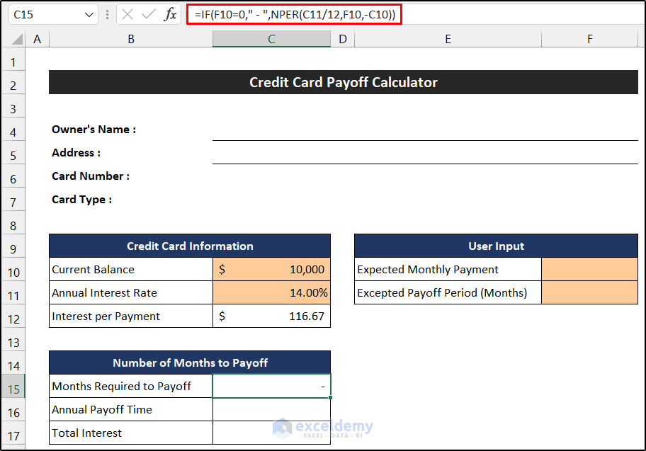
Now, to get the value of the Months Required to Payoff, select cell C15 and write down the following formula into the cell. Here, we are going to use the IF and NPER functions to get the value.

=IF(F10=0," - ",NPER(C11/12,F10,-C10))

Press Enter.

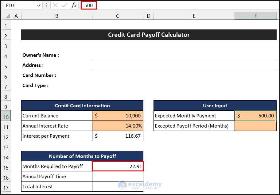
To check the accuracy of our formula, we input $500 in cell F10.
You will see the formula will show us the total number of months.

🔎 Breakdown of the Formula

We are breaking down the formula for cell C15.

👉 NPER(C11/12,F10,-C10): This function returns the total number of periods. Here, the result of this formula is 22.91.

👉 IF(F10=0,” – “,NPER(C11/12,F10,-C10)): Here, the IF function first check the value of the cell F10. If the cell is empty, then the function will return “-”. Otherwise, the function will return the result of the ROUND function.

After that, to convert the result of months into years, write down the following formula into cell C16. Here, we will use the IF and ROUND functions.

=ROUND(C15/12,2)&IF(ROUND(C15/12,2)>1," Years"," Year")

Similarly, press Enter.

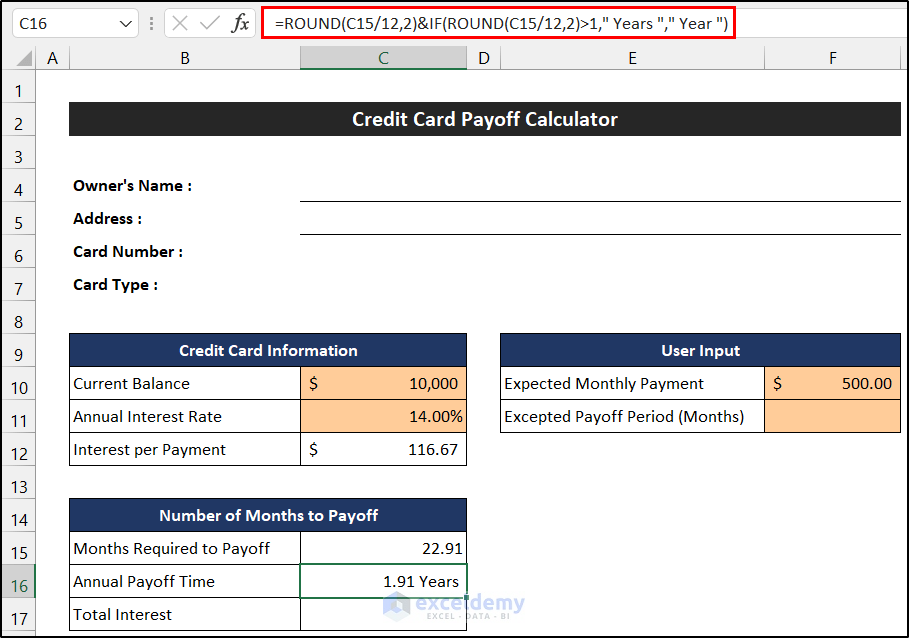
🔎 Breakdown of the Formula

We are breaking down the formula for cell C16.

👉 ROUND(C15/12,2): This function returns the 2-digit rounded value of the result of C15/12. In this case, the result is 1.91.

👉 IF(ROUND(C15/12,2)>1,” Years “,” Year “): Here, the IF function first checks the value of the ROUND function. If the value is greater than 1, then the function will return “ Years”. Otherwise, the function will return “ Year “.

👉 ROUND(C15/12,2)&IF(ROUND(C15/12,2)>1,” Years “,” Year “): The Ampersand operator joins the result of the ROUND and IF function, and shows the result in cell C16.

At last, for estimating the value of the Total Interest, write the following into cell C17. Here, the IF function will help us.

=IF(F10=0," - ",C15*F10-C10)

Again, press Enter.

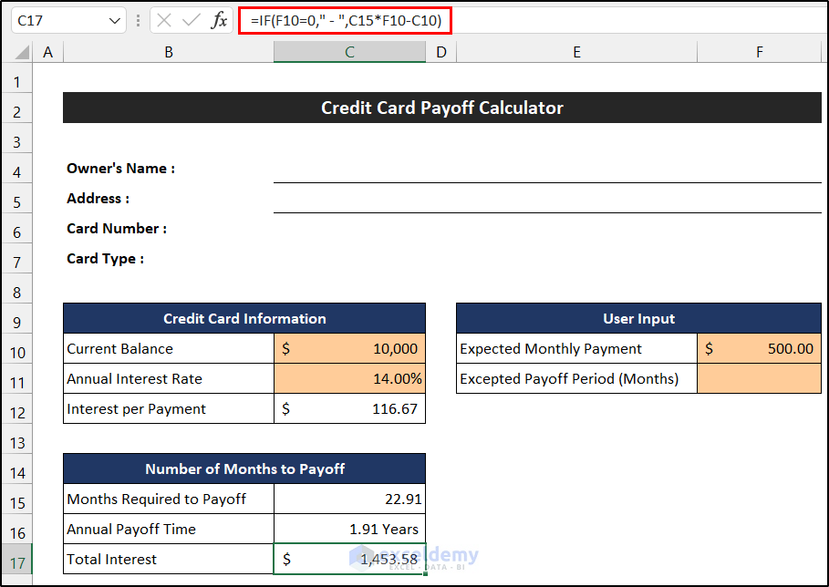
Our job is done, and we are able to get the value of the total months needed to pay off.

Finally, we can say that we have completed the fourth step of creating a pay-off credit card debt calculator in Excel.

Step 5: Calculating Monthly Payment Amount for the Specific Period

In this following step, we will create the section where we will get the monthly payment amount. To get the result from this section, we have to input the desired time period in the month in cell F11.

First of all, write down the title of this section in the merged cell E14.

Now, entitle the following entities in the range of cells E15:E17.

Then, to get the value of the Excepted Payoff Period (Year), select cell F15, and write down the following formula into the cell. Here, we are going to use the IF and ROUND functions to get the value.

=ROUND(F11/12,2)&IF(ROUND(F11/12,2)>1," Years"," Year")

Press Enter.

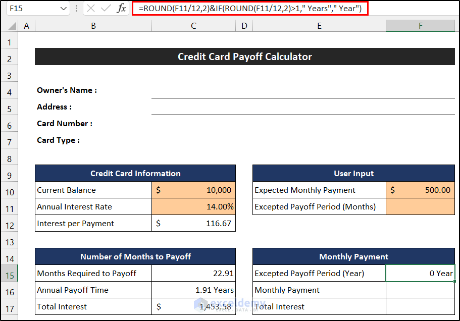
To check the accuracy of our formula, we input 36 in cell F11.
You will see the formula will show us the total number of months.

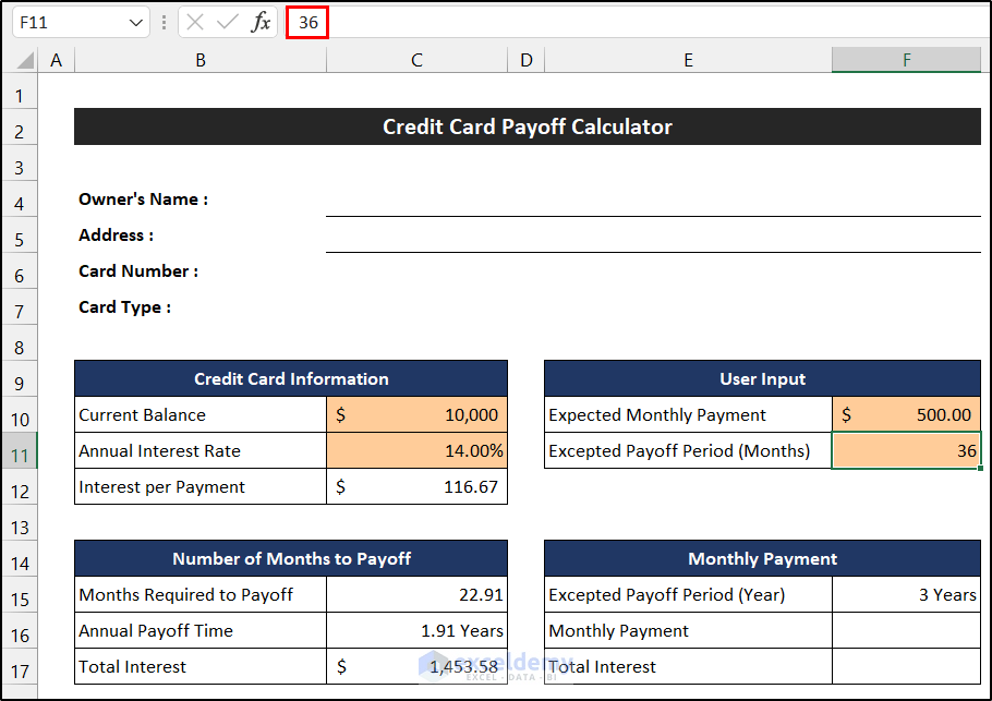
🔎 Breakdown of the Formula

We are breaking down the formula for cell F15.

👉 ROUND(F11/12,2): This function returns the 2-digit rounded value of the result of F11/12. In this case, the result is 3.

👉 IF(ROUND(F11/12,2)>1,” Years”,” Year”): Here, the IF function first checks the value of the ROUND function. If the value is greater than 1, then the function will return “ Years”. Otherwise, the function will return “ Year “.

👉 ROUND(F11/12,2)&IF(ROUND(F11/12,2)>1,” Years”,” Year”): The Ampersand operator joins the result of the ROUND and IF functions, and shows the result in cell F15.

Afterward, to get the value of the monthly payment, write down the following formula into cell F16. Here, we will use the IF and PMT functions.

=IF(F11=0," - ",PMT(C11/12,F11,-C10))

Again, press Enter.

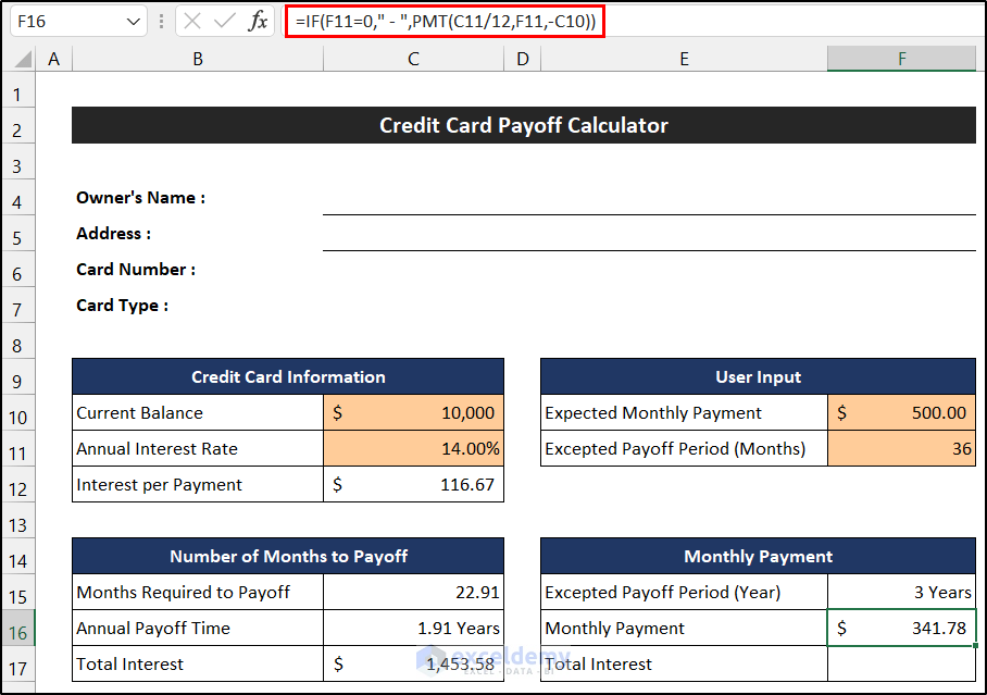
🔎 Breakdown of the Formula

We are breaking down the formula for cell F16.

👉 PMT(C11/12,F11,-C10): This function returns the monthly payment amount. Here, the result of this formula is $341.78.

👉 IF(F11=0,” – “,PMT(C11/12,F11,-C10)): Here, the IF function first checks the value of the cell F11. If the cell is empty, then the function will return “-”. Otherwise, the function will return the result of the PMT function.

In the end, for estimating the value of the Total Interest, write the following into cell F17. Here, the IF function will help us.

=IF(F11=0," - ",F16*F11-C10)

Similarly, press Enter.

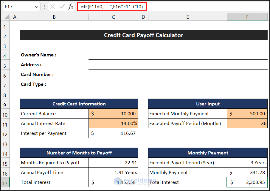
Our job is finished, and we are able to get the amount of the monthly payment.

At last, we can say that we have finished the final step of creating a pay-off credit card debt calculator in Excel.

Step 6: Creating Half Yearly Interval Payment Table in the Credit Card Debt Calculator

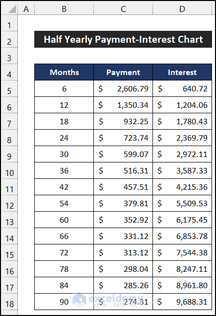
Here, we are going to create a tabular chart where we show the monthly payment and amount of interest. It will help us to explore different types of payment schemes at a time. This step is not mandatory, however, it will provide you with lots of flexibility.

Firstly, create a new sheet.
Next, in the range of cell B5:B6, write down 6 and 12 as the month intervals.

After that, in cell C5, write down the following formula using the PMT function.

=PMT(Calculator!$C$11/12,B5,-Calculator!$C$10)

Press Enter.

Then, write down the following formula into cell D5 to get the total value of the Interest for that scheme.

=(B5*C5)-Calculator!$C$10

Again, press Enter.

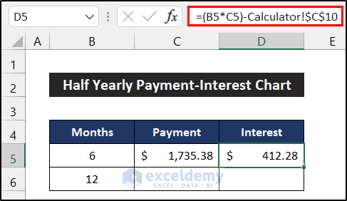
Now, select the range of cells C5:D5 and double-click on the Fill Handle icon to copy the formulas up to row 6.

Finally, select the range of cell B5:D6 and drag the Fill Handle icon according to your desire. You will get the different schemes for every six-month interval. We dragged the Fill Handle icon up to row 18 to show the schemes up to 90 months.
Our half-yearly tabular payment-interest chart is ready.

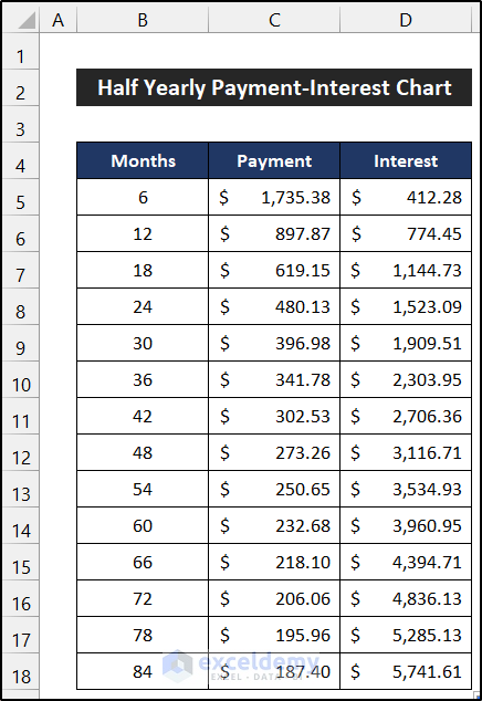
At last, we can say that we have accomplished the payment-interest chart in the template of a pay-off credit card debt calculator in Excel.

Step 7: Establish Relationship Between User Input and Payment-Interest Chart of the Credit Card Debt Calculator

In this step, we are going to establish a relation for checking the payment-interest chart to a cell in the User Input section so that we can browse that table from that section. This step is also not mandatory. Thus, we are showing it to make the calculator more dynamic.

At first, select the range of cells E12:F12.
Now, in the Home tab, click on the Merge & Center option from the group Alignment.

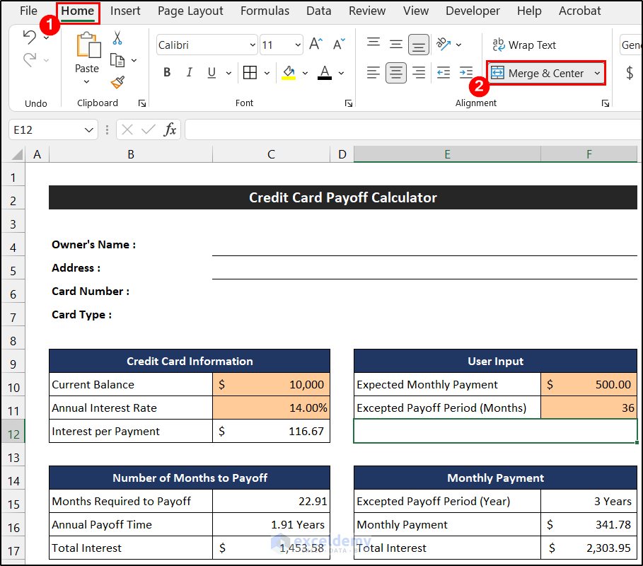
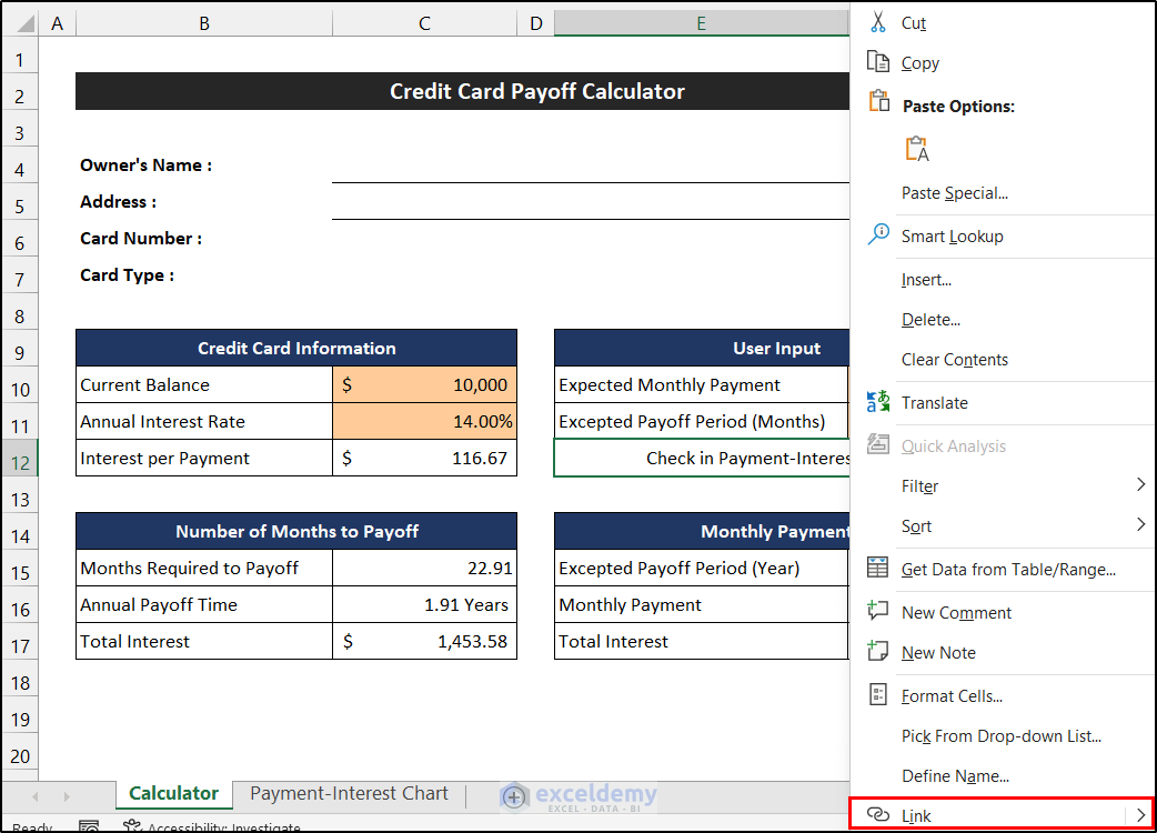
Then, write down a suitable text in the merged cell. We write down the entitlement ‘Check in Payment-Interest Chart’.

Afterward, Right-Click on the cell, and from the Context Menu, choose the Link option.

As a result, a small dialog box called Insert Hyperlink will appear.
In the Link to field, select the Place in This Document option and choose the sheet entitled Payment-Interest Chart.
Finally, click OK.

You will notice that a browsing link of the Payment-Interest Chart sheet will insert in that cell.

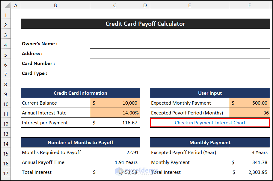
At last, format the cell according to your wish.

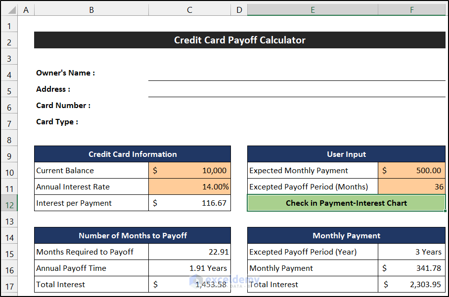
The relation establishment task is finished. Now, if you click on the text of cell E12, you will directly go to the Payment-Interest Chart sheet.

Thus, we can say that we have completed a relation establishment task in the template of a pay-off credit card debt calculator in Excel.

Step 8: Verifying Pay off Credit Card Debt Calculator in Excel with Sample Data

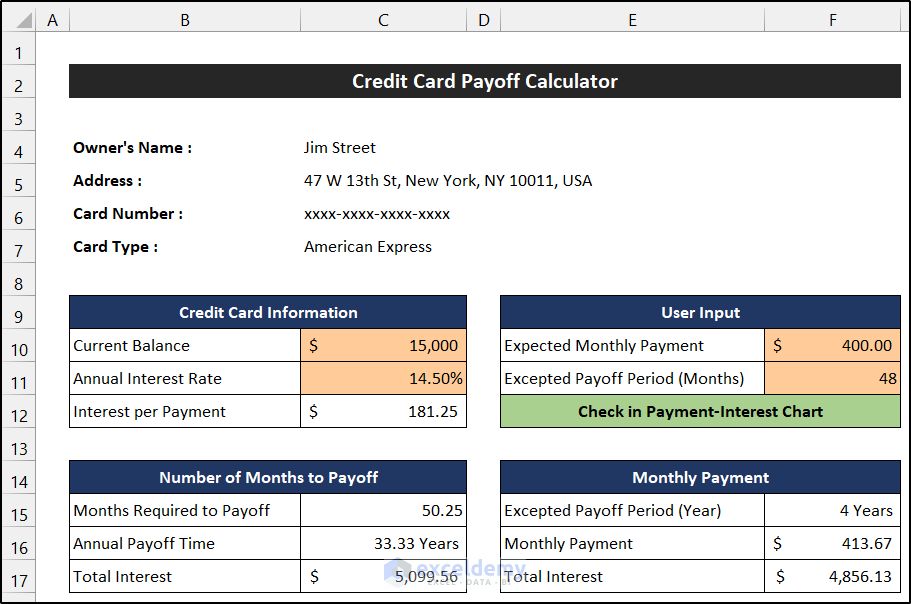
Now, we will check the accuracy of our calculator with a new sample dataset. Our sample dataset is shown as follows:

1. 1. 1. 1. Owner’s Name: Jim Street
        
        Address: 47 W 13th St, New York, NY 10011, USA
        
        Card Number: xxxx-xxxx-xxxx-xxxx
        
        Card Type: American Express
        
        Current Balance: $15,000
        
        Annual Interest Rate: 14.50%
        
        Expected Monthly Payment: $400
        
        Excepted Payoff Period (Months): 48

Now, input this sample dataset into the calculator.

You will notice the calculator will show new values for paying off this loan.

In addition, if you click the Check in Payment-Interest Chart text of cell E12, you can explore other schemes also.

Finally, we can say that all of our tasks are completed, and we are able to create a pay-off credit card debt calculator in Excel.

Download Free Templates

Download this free template while you are reading this article.

Pay off Credit Card Debt Calculator.xlsx

Conclusion

That’s the end of this article. I hope that this article will be helpful for you and you will be able to create pay off credit card debt calculator in Excel. Please share any further queries or recommendations with us in the comments section below if you have any further questions or recommendations.

<< Go Back to Debt Template | Finance Template | Excel Templates

Get FREE Advanced Excel Exercises with Solutions!