Method 1 – Using the PMT Function to Calculate Annuity Payments
Steps:
- Select cell C9 where you want to calculate the Annual Investment.
- Enter the corresponding formula in the C9 cell:
=PMT(C6,C7,0,C5)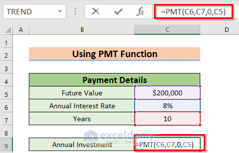
Formula Breakdown
Here, I have used the PMT function, which calculates the payment based on an Annuity with a constant interest rate and regular investment.
- In this function, C6 denotes the Annual Interest Rate of 8%.
- C7 denotes the total payment period in terms of the year, which is 10.
- 0 denotes the present value.
- C5 denotes the Future Value, which is $200,000.
- Press ENTER to get the Annual Investment.
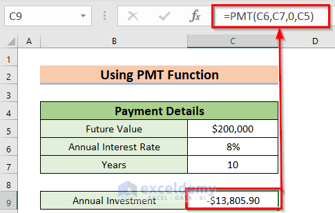
Here, the Minus sign denotes that you must pay this amount to the insurance company. This means Annual Investment is an outgoing monetary amount. Now, I will change the format.
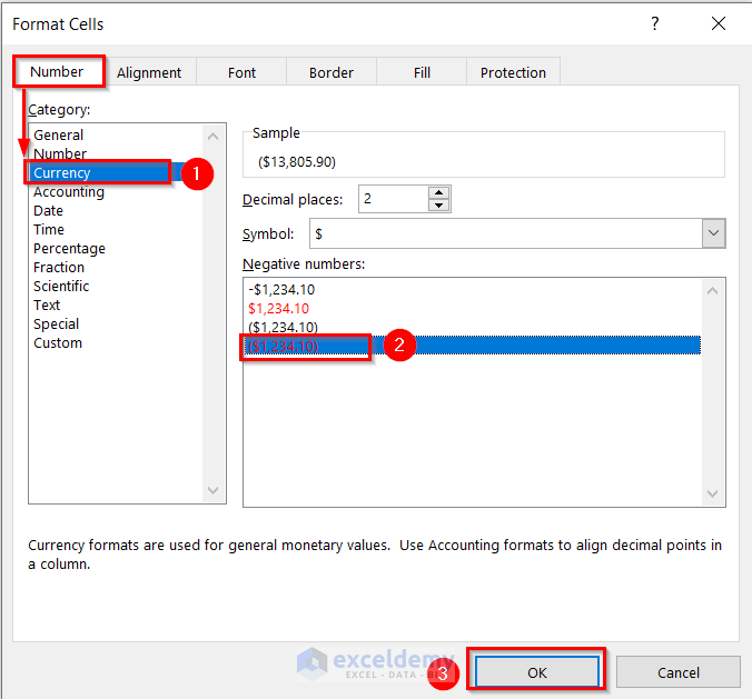
- Press the CTRL+1 to open the Format Cells dialog box.
You can also use the Context Menu Bar or the Custom Ribbon to go to the Format Cells command.
- If you are using the Context Menu Bar, select the data range >> Right-click on the data >> choose the Format Cells option.
- If you are using Custom Ribbon, select the data range >> from the Home tab >> go to the Format feature >> choose the Format Cells command.
A dialog box named Format Cells will appear.
- Make sure that you are using the Number command.
- Go to the Currency option.
- Choose the fourth option from the Negative numbers option.
- Press OK.
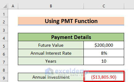
You will see the following result.
Method 2 – Applying PV Function to Calculate Annuity Payments
Steps:
- Select a cell (C9) where you want to calculate the Total Investment.
- Enter the corresponding formula in the C9 cell:
=PV(C6,C7,C5,,0)- Press ENTER to get the Total Investment.

Formula Breakdown
Here, the PV function will return the Present Value of an investment.
- C6 denotes the rate as the annual interest rate.
- C7 denotes NPER as the total period of time.
- C5 denotes the PMT as an Annuity Payment.
- As the Future Value is unknown FV will be Blank.
- 0 denotes Types as the ending of the period.
Read More: How to Calculate Annuity Factor in Excel
Method 3 – Using the FV Function to Calculate Annuity Payments
Steps:
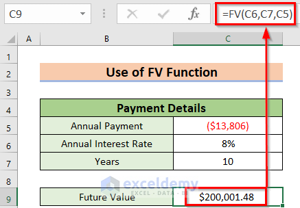
- Select a cell (C9) where you want to calculate the Annuity Payment, the Future Value.
- Enter the corresponding formula in the C9 cell:
=FV(C6,C7,C5)- Press ENTER to get the Future Value.
Formula Breakdown
- Here, the FV function will return a Future Value of the periodic investment.
- Now, C6 denotes the Annual Interest Rate.
- Then, C7 denotes the total time period as Year.
- Finally, C5 denotes the monetary value that you are paying at present annually to get an Annuity Payment in the future.
Read More: How to Calculate Deferred Annuity in Excel
Method 4 – Employing Generic Formula to Calculate Annuity Payments
Steps:
- Select a cell (C9) where you want to calculate the Total Investment.
- Enter the corresponding formula in the C9 cell:
=C5*((1-(1+C6)^-C7)/C6)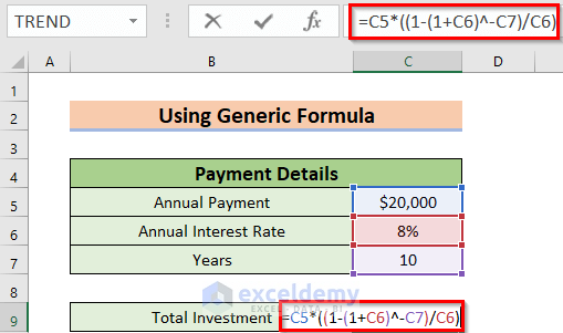
Formula Breakdown
- Here, C6 denotes the Annual Interest Rate.
- Firstly, I have added 1 with the interest rate.
- Output: 1.08.
- Secondly, the Power (^) sign raises it to a fixed power, which is the negative value of the C7 cell. Also, that is the time period.
- Output: 0.463193488.
- Thirdly, I have subtracted the above output from 1.
- Output: 0.536806512.
- Fourthly, I have divided the above result by C6, which is the Annual Interest Rate.
- Output: 6.710081399.
- Here, C5 denotes the monetary value you will receive annually, which means this is the Annuity Payment.
- Finally, I have multiplied the C5 cell value with the above result.
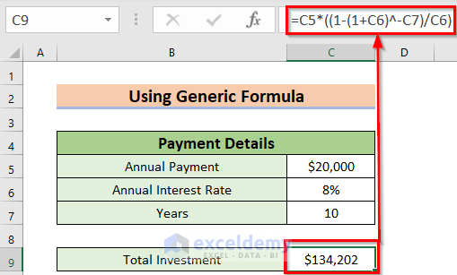
- Output: $134,201.63.
- Press ENTER to get the Total Investment.
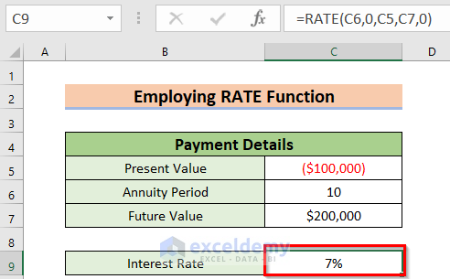
Calculating the Interest Rate of Annuity Payments by Using the RATE Function
Steps:
- Select a cell (C9) where you want to calculate the Interest Rate.
- Enter the corresponding formula in the C9 cell:
=RATE(C6,0,C5,C7,0)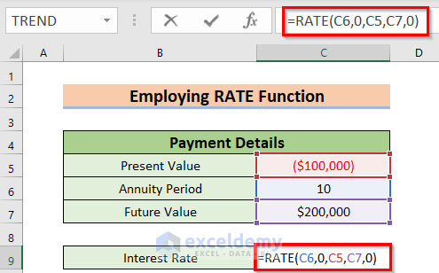
Formula Breakdown
Here, the RATE function will return the annual rate in percentage of investment.
- Now, C6 denotes the NPER as the annuity period.
- Then, 0 denotes that the annual payment is unknown.
- Then, C5 denotes the total investment that you will pay today to the insurance company.
- After that, C7 denotes the equivalent Future value you will get after the annuity period.
- Finally, 0 denotes the type as the ending of the period.
- Press ENTER to get the Interest Rate.
Employing the NPER Function to Calculate the Annuity Period
Steps:
- Select a cell (C9) where you want to calculate the Interest Rate.
- Enter the corresponding formula in the C9 cell:
=NPER(C6,C7,C5,,0)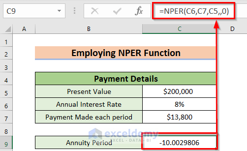
Formula Breakdown
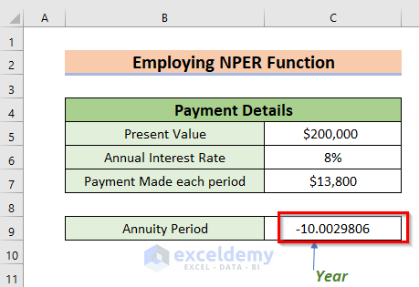
Here, the NPER function gives the payment period as a year.
- C6 denotes the Annual Interest Rate.
- C7 denotes how much you are paying per period.
- C5 denotes the total investment that you make in the insurance company.
- As the Future Value is unknown FV will be Blank.
- 0 denotes the type as the ending of the period.
- Press ENTER to get the Annuity Period.
Things to Remember
- There is one more feature to the RATE function, which is a guess. Basically, the RATE function will do a maximum of 20 iterations. So, this function has to do more than 20 iterations when it does not give a result. In that case, you have to guess the interest rate.
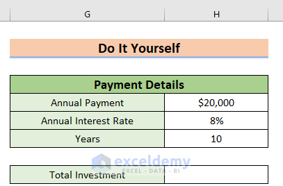
Practice Section
Now, you can practice the explained method.
Download the Practice Workbook
You can download the practice workbook from here:
Related Articles
<< Go Back to Excel Annuity Formula | Excel Formulas for Finance | Excel for Finance | Learn Excel
Get FREE Advanced Excel Exercises with Solutions!

