In this article, we will demonstrate how to create a multiple credit card payoff calculator spreadsheet in Excel.
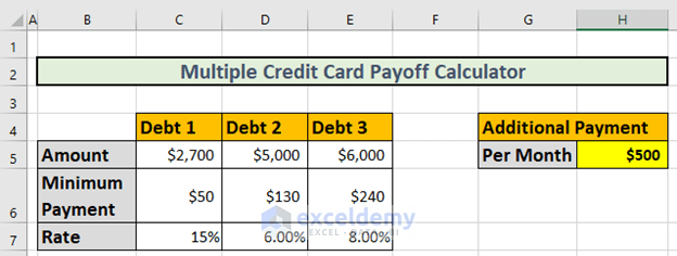
We’ll use the dataset below containing 3 debts, and create a payoff schedule for these loans.
Please note that we will follow the debt snowball method.
As per the debt snowball method:
- First of all, we have to pay a minimum amount for each loan.
- We will make an additional payment to pay off the lowest debt.
- After repaying the lowest debt, we will continue the additional payment to pay off the 2nd lowest debt, and so on.
The minimum payments for each loan are in the dataset. We will additionally pay $500 per month to repay the loans.
Step 1 – Calculate the Payment for Each Debt for the First Month
We will apply different formulas for each debt.
1.1 – Calculating the Lowest Debt
First of all, we will determine the payment for the 1st month for the lowest debt using the IF function.
- Go to cell C11 and enter the following formula:
=IF(H5>=C5,C5,H5+C6)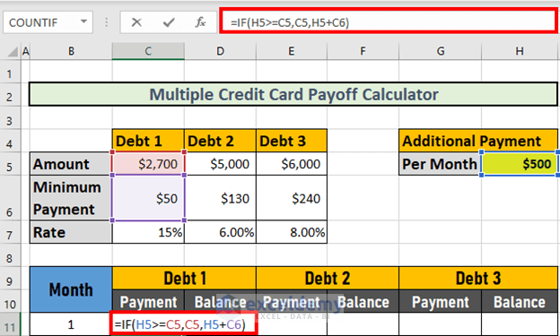
- Press ENTER to return the output.
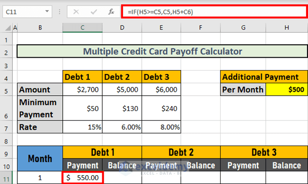
Explanation:
Since $500 < $2700, the logical statement is FALSE. So the output is H5+H6 = $550.
1.2 – Second Lowest Debt Calculation
Now, we will create a formula for the payment in the 1st month for the 2nd lowest debt, that is debt-2, using a combination of the IF and AND functions.
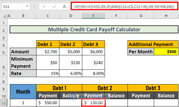
- Go to cell E11 and enter the following formula:
=IF(H5>=C5+D5,D5,IF(AND(C11=C5,C11<>0),H5-D5+D6,D6))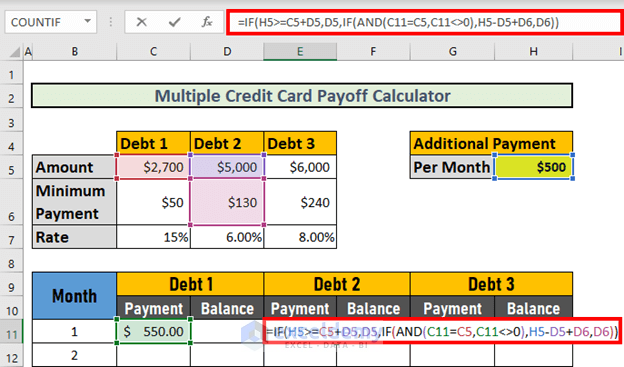
Formula Breakdown:
- AND(C11=C5,C11<>0)
- Output: FALSE
- IF(AND(C11=C5,C11<>0),H5-D5+D6,D6)
- Output: 130
- IF(H5>=C5+D5,D5,IF(AND(C11=C5,C11<>0),H5-D5+D6,D6)) resolves to:
- IF(FALSE,5000,130)
- Output: 130
- Press ENTER to calculate the payment.
1.3 – Last Debt Calculation
Now we’ll calculate the payment in the 1st month for the last debt using a similar formula.
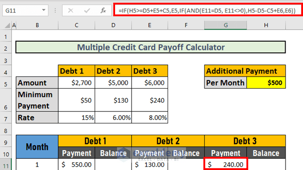
- Go to cell G11 and enter the following formula:
=IF(H5>=D5+E5+C5,E5,IF(AND(E11=D5, E11<>0),H5-D5-C5+E6,E6))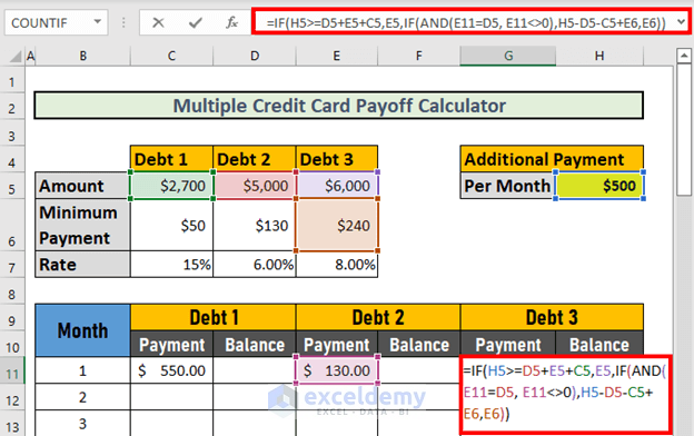
Formula Breakdown:
- AND(E11=D5, E11<>0)
- Output: FALSE
- IF(AND(E11=D5, E11<>0),H5-D5-C5+E6,E6)
- Output: 240
- IF(H5>=D5+E5+C5,E5,IF(AND(E11=D5, E11<>0),H5-D5-C5+E6,E6)) resolves to:
- IF(FALSE,6000,240)
- Output: 240
- Press ENTER to return the result.
Step 2 – Determining the Remaining Balance of Each Debt After the First Month
2.1 – Lowest Debt Calculation
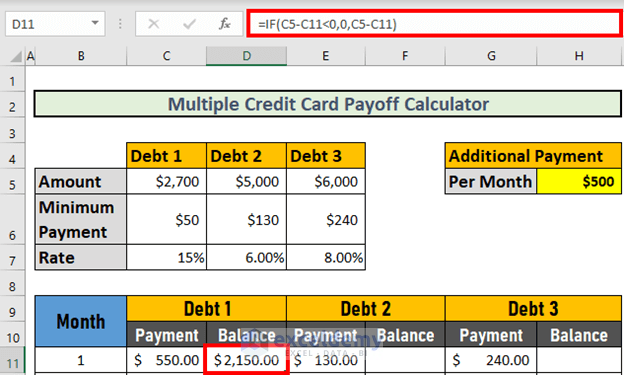
To determine the remaining balance of the lowest debt (that is debt-1) after the 1st month:
- Go to cell D11 and enter the following formula:
=IF(C5-C11<0,0,C5-C11)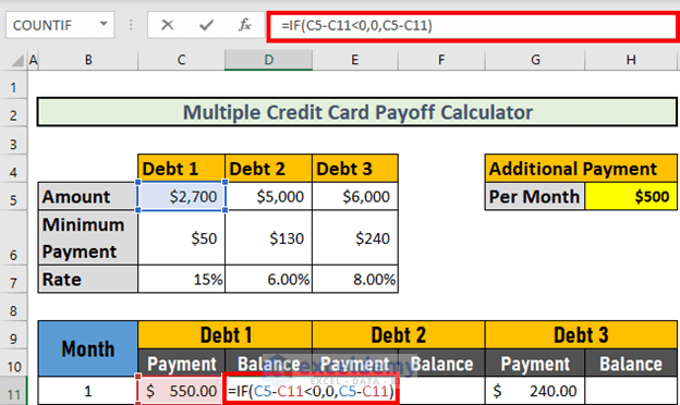
- Press ENTER to return the result.
2.2 – Second Lowest Debt Calculation
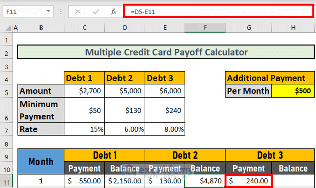
To calculate for debt-2, we will simply subtract the 1st month’s payment from the total amount due.
- Go to cell F11 and enter the following formula:
=D5-E11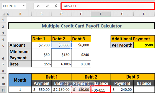
- Press ENTER to return the result.
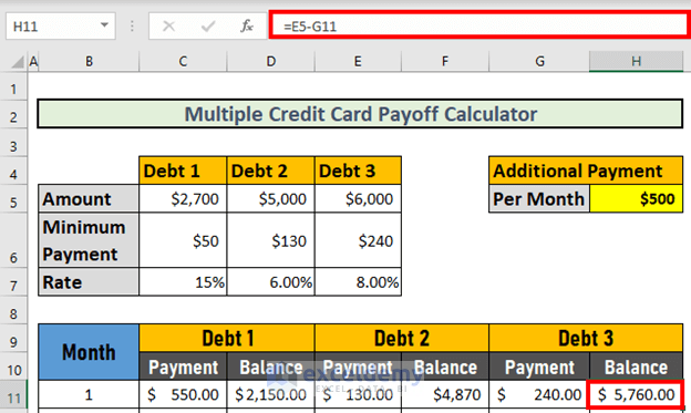
2.3 – Last Debt Calculation
We calculate the remaining balance for debt-3 in the same way:
Step 3 – Calculating the Payment of Each Debt for the Next Months
Now we can calculate the payment of each debt for the subsequent months. The formulas are different from those used for the 1st month.
3.1 – Lowest Debt Calculation
To calculate the lowest debt i.e. debt-1:
- Go to cell C12 and enter the following formula:
=IF(D11-$H$5-$C$6<=0,$H$5+D11-$H$5,$H$5+$C$6)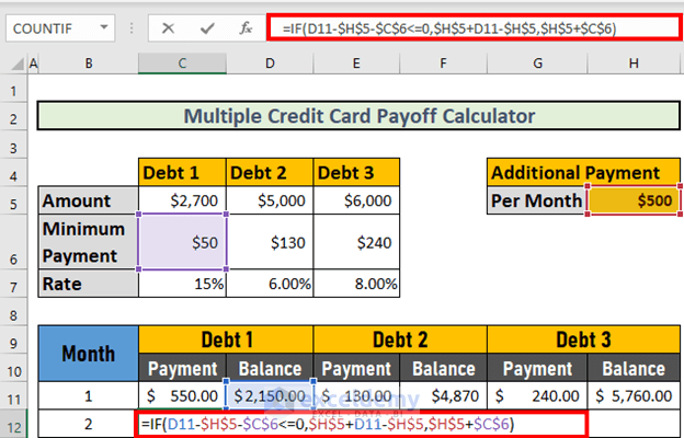
Formula Breakdown:
- D11-$H$5-$C$6<=0
- Output: FALSE
- IF(D11-$H$5-$C$6<=0,$H$5+D11-$H$5,$H$5+$C$6) resolves to:
- IF(FALSE,2150,550)
- Output: 550
- Press ENTER to return the result.
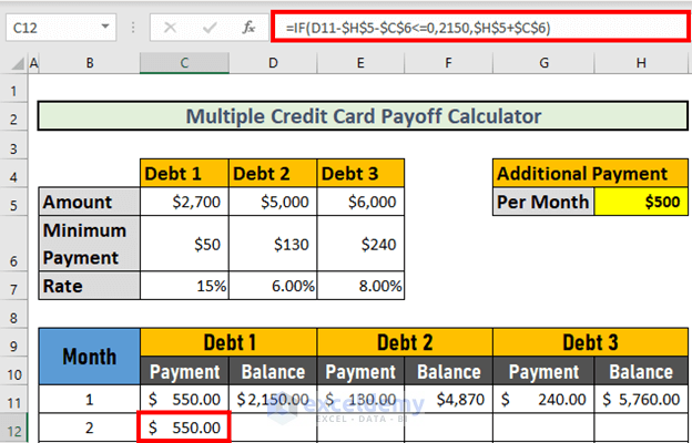
3.2 – Second Lowest Debt Calculation
To calculate the payment for debt-2, we’ll use a combination of the AND and IF functions.
- Go to cell E12 and enter the following formula:
=IF(AND(((F11-$H$5+C12-D$6-C$6)<=0),D12=0),F11,IF((F11-$D$6-$H$5)<=0,F11,IF(D12=0,$H$5-C12+D$6,D$6)))
Formula Breakdown:
- IF(D12=0,$H$5-C12+D$6+C$6,D$6)
- Output: 130
- (F11-$D$6-$H$5)<=0
- Output: FALSE
- IF((F11-$D$6-$H$5)<=0,F11,IF(D12=0,$H$5-C12+D$6+C$6,D$6)) resolves to:
- IF(FALSE,4870,130)
- Output: 130
- AND(((F11-$H$5+C12-D$6-C$6)<=0),D12=0)
- Output: FALSE
- IF(AND(((F11-$H$5+C12-D$6-C$6)<=0),D12=0),F11,IF((F11-$D$6-$H$5)<=0,F11,IF( D12=0,$H$5-C12+D$6,D$6))) resolves to:
- IF(FALSE,4870,130)
- Output: 130
- Press ENTER to return the result.
3.3 – Last Debt Calculation
We create another formula to give us the payment for the subsequent months for debt-3.
- Go to cell G12 and enter the following formula:
=IF(AND(((H11-$H$5+E12-E$6-D$6-C$6)<=0),F12=0),H11, IF((H11-$E$6-$H$5)<=0,H11,IF(F12=0,$H$5-E12+E$6,E$6)))
Formula Breakdown:
- IF(F12=0,$H$5-E12+E$6+D$6+C$6,E$6)
- Output: 790
- (H11-$E$6-$H$5)<=0
- Output: FALSE
- IF((H11-$E$6-$H$5)<=0,H11,IF(F12=0,$H$5-E12+E$6+D$6+C$6,E$6)) resolves to:
- IF(FALSE,5760,790)
- Output: 790
- AND(((H11-$H$5+E12-E$6-D$6-C$6)<=0),F12=0)
- Output: FALSE
- =IF(AND(((H11-$H$5+E12-E$6-D$6-C$6)<=0),F12=0),H11, IF((H11-$E$6-$H$5)<=0,H11,IF(F12=0,$H$5-E12+E$6,E$6))) resolves to:
- IF(FALSE,5760,790)
- Output: 790
- Press ENTER to return the result.
Note: This amount is not the correct one. However, the formula is correct. Once we calculate the remaining balances (shown in subsequent steps), we will get the accurate amount.
Step 4 – Determining the Remaining Balance of Each Debt for the Next Months
Now, we will calculate the remaining balances of these debts for the next few months, considering the interest applied to the remaining balances.
4.1 – Lowest Debt Calculation
First, we create a formula for debt-1.
- Go to cell D12 and enter the following formula:
=IF(D11-C12<=0,0,(D11-C12)*(1+($C$7/12)))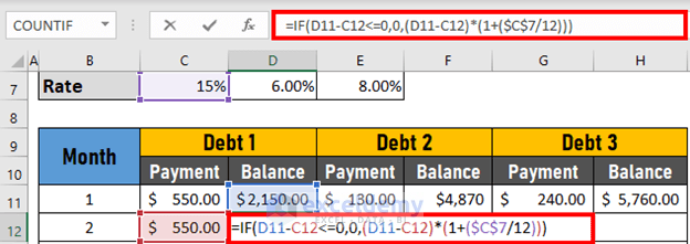
Formula Breakdown:
- (D11-C12)*(1+($C$7/12)) → ($C$7/12) is the monthly interest rate.
- Output: 1620
- D11-C12<=0
- Output: FALSE
- =IF(D11-C12<=0,0,(D11-C12)*(1+($C$7/12))) resolves to:
- IF(FALSE,0,1620)
- Output: 1620
- Press ENTER to return the result.
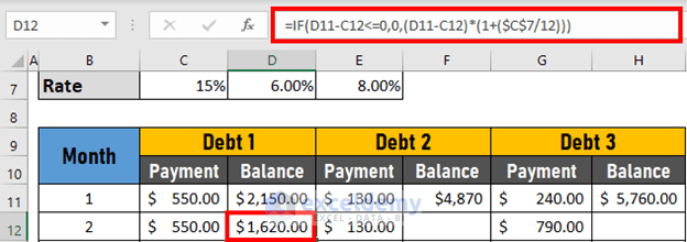
4.2 – Second Lowest Debt Calculation
- Go to cell F12 and enter the following formula:
=IF(F11-E12<0,0,(F11-E12)*(1+($D$7/12)))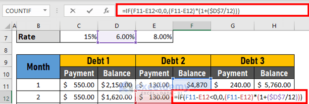
- Press ENTER to return the result.
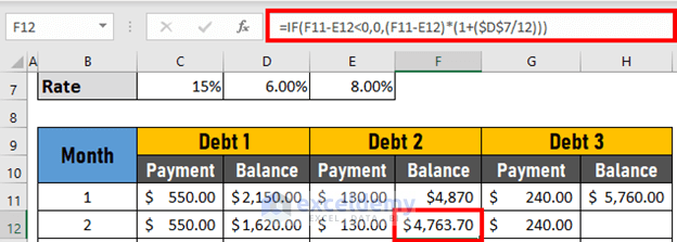
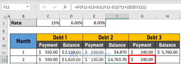
Note: As soon as we calculate the balance for debt-2, the accurate payment appears for debt-3. The payment is $240 now, where previously it was $790.
4.3 – Last Debt Calculation
- Go to cell H12 and enter the following formula:
=IF(H11-G12<0,0,(H11-G12)*(1+($E$7/12)))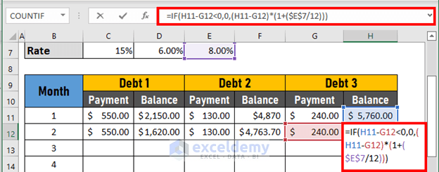
- Press ENTER to return the result.
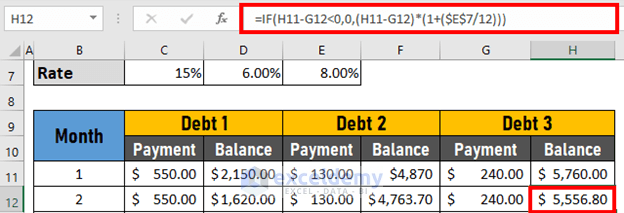
Step 5 – Using AutoFill to Create a Calculator
Finally, we’ll use the Fill Handle and AutoFill to complete the calculator.
- Use the AutoFill feature on the Payment column of debt-1.
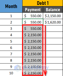
The values are not correct. However once we AutoFill all the columns, the exact values will appear.
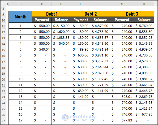
Read More: How to Create a Credit Card Payoff Spreadsheet in Excel
Things to Remember
- Remember to repay a minimum amount on all the loans.
- Use an absolute reference to lock a cell.
Download Practice Workbook
Related Articles
- How to Create Credit Card Payoff Calculator with Snowball in Excel
- Make Credit Card Payoff Calculator with Amortization in Excel
<< Go Back to Credit Card Payoff Calculator | Finance Template | Excel Templates
Get FREE Advanced Excel Exercises with Solutions!


Having difficulty adding Debt 4 and Debt 5 formula is confusing me
Hi Ketayla!
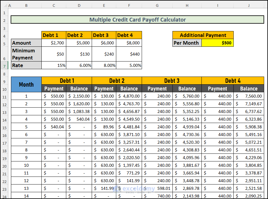
Thanks for the comment. There were some errors in the formula of Lowest Debt Calculation and I have fixed it. Also for your convenience, I have added the debt 4 in the workbook. Following the same method, you can create a formula yourself for debt 5, debt 6, and more. You can download the file from this link.
Here is the image of the solution:
Thanks for supporting us! If you face any other problem with any other topic then reply in the comment section.
This does not take interest added each month into the balances due. Do you have a solution?
Hello Patricia,
To solve this issue:
First, add columns for monthly interest and new balance.
Then, for each debt, include columns for monthly interest and new balance.
Use the following formula to calculate monthly interest:
Monthly Interest = Previous Balance * (Annual Interest Rate / 12)
Example:
Debt 1 (D2): =C2*0.17/12
Debt 2 (H2): =G2*0.19/12
Debt 3 (L2): =K2*0.20/12
Use the following formula to calculate new balance:
New Balance = Previous Balance + Monthly Interest – Payment
Example:
Debt 1 (E2): =C2+D2-B2
Debt 2 (I2): =G2+H2-F2
Debt 3 (M2): =K2+L2-J2
Regards
ExcelDemy
adding debt 5 is confusing. Can you help please
Hello Lacy,
To add “Debt 5” to the multiple credit card payoff calculator, you need to copy the structure for the previous debts. Simply add a new row for Debt 5 and input the same type of information as the other debts, such as balance, interest rate, and monthly payment. Ensure that all the formulas used for the other debts are also applied to Debt 5, especially in the summary and payoff sections.
Regards
ExcelDemy