How to Lock Table Array in Excel (2 Effective Ways)

In this tutorial, I am going to show you 2 effective ways how to lock table array in Excel. You can apply these methods to any type of dataset and lock them in a short amount of time. Also, in the last section, I will show you a quick way to lock and protect your data table from alterations.

Why Do We Need to Lock Table Array?

In many cases, we need to apply a specific formula to a large number of cells where the formula references a certain table. What happens is that the formula of the first cell seems to work properly. But for the other cells, it may fail to give the expected values. In such situations, we have to lock the table reference inside the formula in Excel so that they work accurately.

Read More: What Is Table Array in Excel VLOOKUP?

How to Lock Table Array in Excel: 2 Effective Ways

For this tutorial, we have a dataset with 2 tables. The first table has the name of the students and their marks. The second one has the criteria to set a specific grade for each mark range. We will lock table array in Excel using the below dataset.

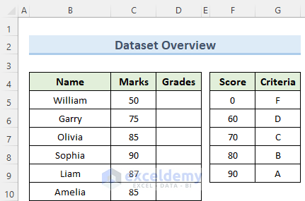
1. Using Absolute Referencing in VLOOKUP Function to Lock Table Array in Excel

The VLOOKUP function in Excel looks up values in a table that is organized vertically. We can use this function to reference and lock a table array in Excel easily. Follow the steps below to do this.

Steps:

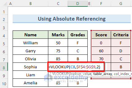
• First, double-click on cell D5 and enter the below formula:

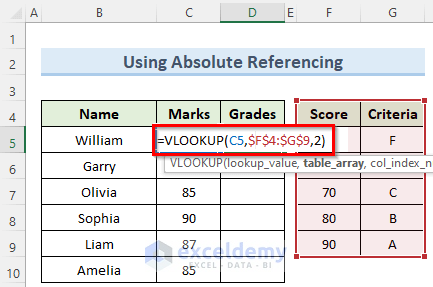
• Then, press Enter and you should see the result that the formula has referenced from the Criteria table.

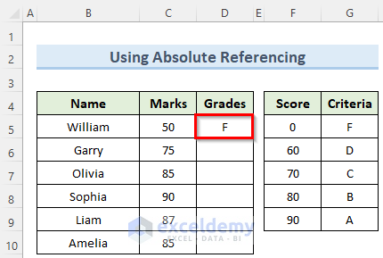
• Now, copy the above formula to the cells below using the Fill Handle.

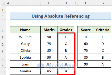
• Finally, you can confirm that the formula has locked the reference table by double-clicking on cell D8.
• As you can see, the table range is constant for the remaining cells as well.

2. Defining Range Name Inside VLOOKUP Function

As we have seen in the previous method, we can set a table range inside the VLOOKUP function. Another way we can specify a table in the formula is by using the Define Name feature in Excel. Using this feature, we can speed up the process to lock the table array in Excel. Let us see how to apply this.

Steps:

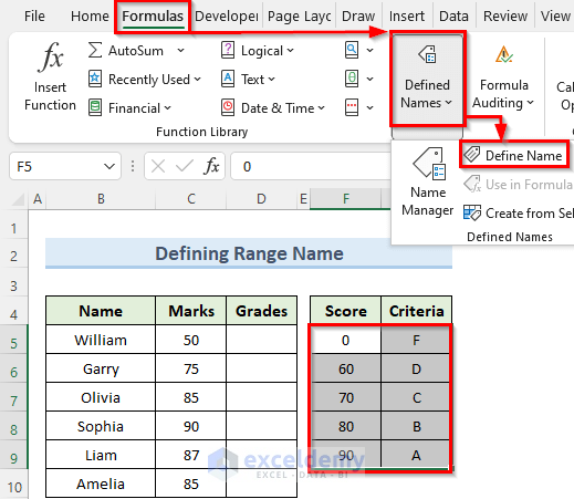
• To begin with, select the table that you want to lock in the VLOOKUP.
• Note that, you should not select the table headers.
• Now, go to the Formulas tab and then to the section Defined Names.
• There, click on Define Name.

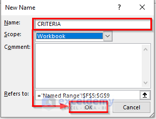
• Next, in the New Name window, type a name in the field Name.
• Then select OK.

• Now, double-click on cell D5 and type in the following formula:

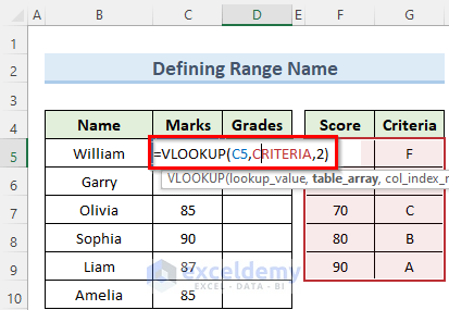
• Then, press the Enter key and this will reference the value F from the second table.

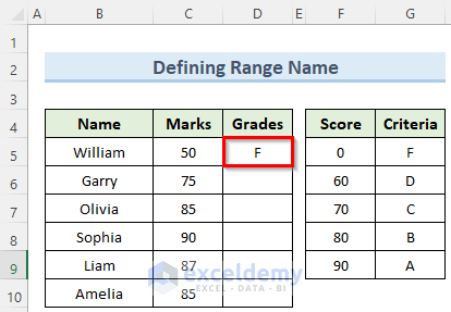
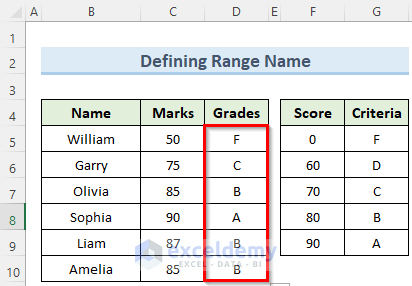
• After that, copy the formula to the remaining cells below using Fill Handle.
• Consequently, you can notice that Grades values are coming from the same range that we specified which means it is locked by the formula.

Read More: How to Name a Table Array in Excel

How to Lock Table Data Using Protect Sheet Option in Excel

If you want to protect a specific data table in an Excel worksheet, then you can apply this method. This will enable you to lock all the cells inside the table from changing without permission. See the steps below.

Steps:

• To start with, select the whole dataset including the headers.

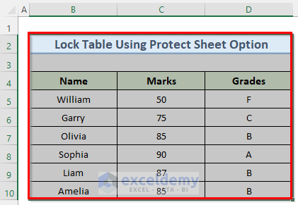
• Now, right-click on the dataset and select Format Cells.

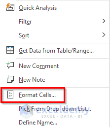
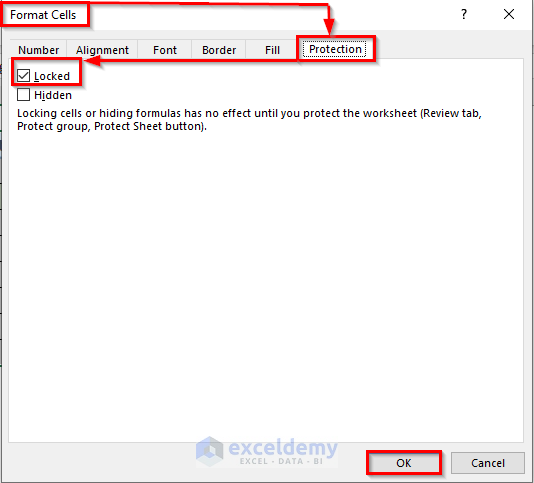
• Next, in the Format Cells window, go to the Protection tab and check the option Locked.
• After that click OK.

• Then, while you have the dataset selected, navigate to the Review tab and select Protect Sheet.

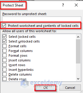
• Here, in the Protect Sheet window, check the option Protect worksheet and contents of locked cells and select OK.
• As a result, excel will lock your whole data table from making any changes to the contents.

Read More: How to Expand Table Array in Excel

Things to Remember

• Instead of manually typing the $ sign, you can also select the table range inside the formula and then press F4.
• Make sure to organize the data in the Criteria table in ascending order going down.
• The third parameter in the formula having a value of 2, denotes the index number of the Marks column of the first table.

Download Practice Workbook

You can download the practice workbook from here.

Conclusion

I hope that you understood the methods on how to lock table array in Excel and were able to apply them properly. If you get stuck in any of the steps, I recommend going through the tutorial a few times so that you understand them very well. Also, download the practice workbook and change the table to make it more challenging.

Related Articles

• How to Use VLOOKUP Table Array Based on Cell Value in Excel
• How to Find Table Array in Excel

<< Go Back to Table Array in Excel | Excel VLOOKUP Function | Excel Functions | Learn Excel