How to Make an Electronic Raffle Draw in Excel (2 Ways)

To select a winner from a lottery, a raffle draw is required. Drawing raffles manually is time-consuming and tedious if there are many participants. But this process becomes easier if we do an electronic raffle draw using Microsoft Excel.

In this article, we’ll demonstrate two different methods to accomplish this. We will nest the RANDBETWEEN function with the INDEX function in our first method. And for our second approach, we will combine the INDEX function with the MATCH function.

For our two procedures, we will use the following data set.

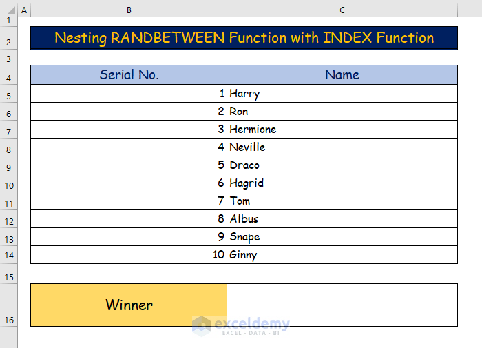
Method 1 – Nesting RANDBETWEEN Function with INDEX Function

The RANDBETWEEN function will generate a random number from the data set. Then the INDEX function will derive the name that is associated with that random number.

Steps:

Insert the following nested formula in cell C16:

=INDEX(C5:C14,RANDBETWEEN(1,10))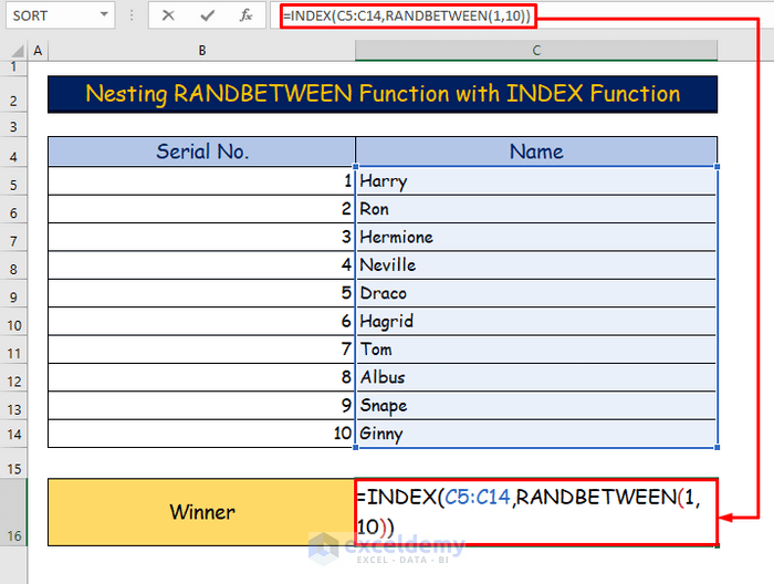

Formula Breakdown

RANDBETWEEN(1,10): The RANDBETWEEN function generates a random number from 1 to 10. As we have 10 entries in our data set, it takes 1 as the lower limit and 10 as the upper limit.
INDEX(C5:C14,RANDBETWEEN(1,10)): Then, the INDEX function returns the name that is associated with the randomly selected number.

Press Enter.
The winner’s name, randomly selected by our functions, appears.

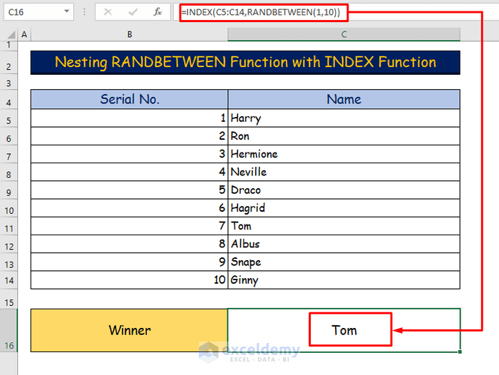
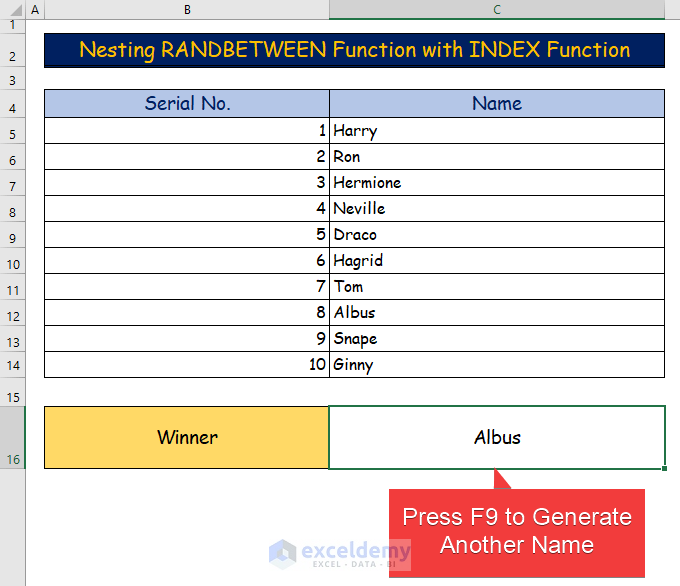
Furthermore, by pressing F9 on the keyboard, you can automatically generate more names.

Method 2 – Combining INDEX and MATCH Functions

This method combines the INDEX function and the MATCH function, along with the MAX function and the MIN function. This method is applicable if you have a set of values assigned to each raffle holder and want to decide the winner based on those values.

2.1 – Draw the Maximum Value from the Raffle

Steps:

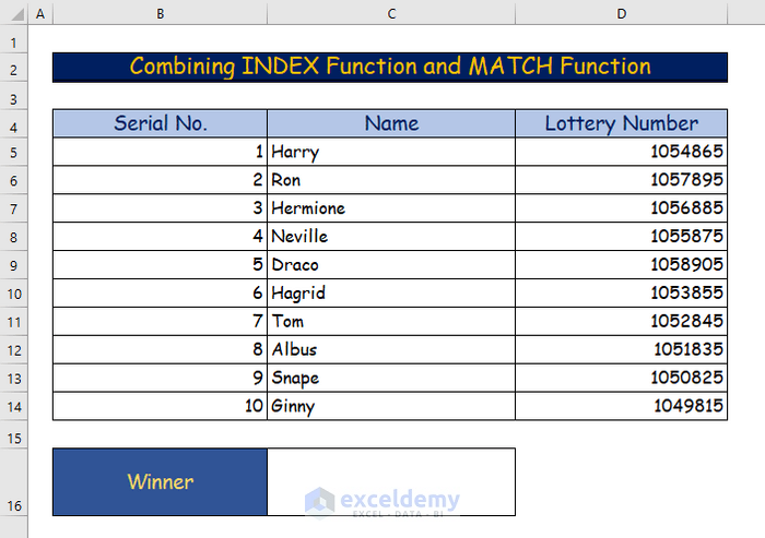
Add an extra table to our dataset to display lottery numbers.

Enter the following formula in cell C16:

=INDEX(C5:C14,MATCH(MAX(D5:D14),D5:D14,0))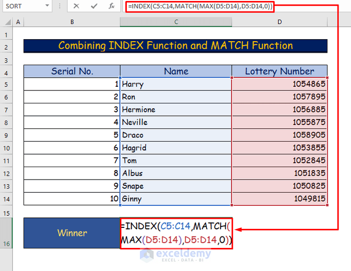

Formula Breakdown

MAX(D5:D14): The MAX function finds the maximum value from the cell range D5:D14.
MATCH(MAX(D5:D14),D5:D14,0): The MATCH function searches for the location of that maximum value, returning an exact match.
INDEX(C5:C14,MATCH(MAX(D5:D14),D5:D14,0)): The INDEX function takes the location range from the MATCH function and returns the name associated with the result with the maximum value.

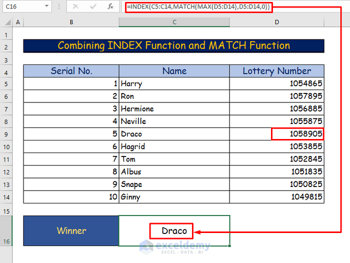
Press Enter button to return the result.
The winner is Draco, who holds the lottery number with the highest value.

2.2 – Draw the Minimum Value from the Raffle

Steps:

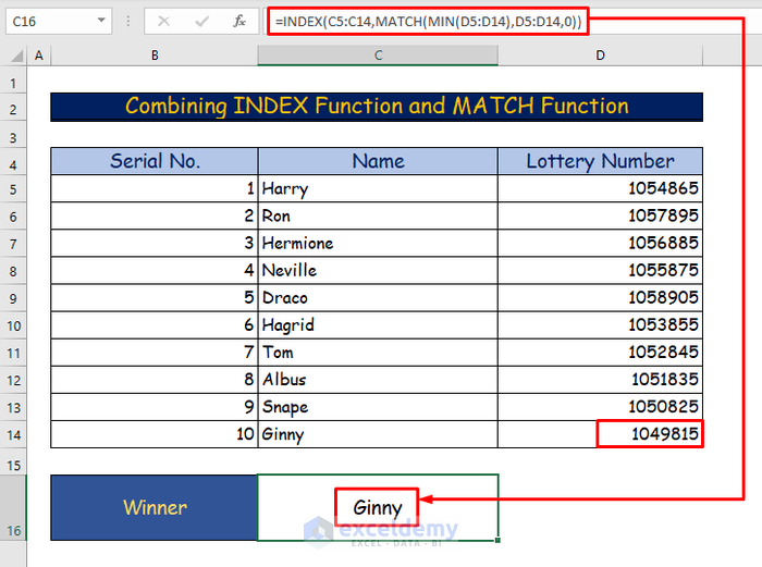
Enter the following formula in cell C16:

=INDEX(C5:C14,MATCH(MIN(D5:D14),D5:D14,0))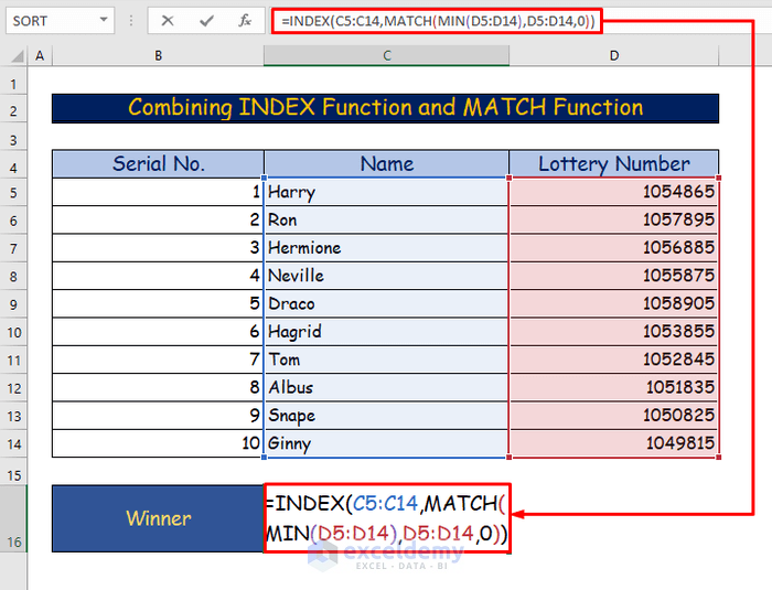

Formula Breakdown

MIN(D5:D14): The MIN function will search for the minimum value in the cell range D5:D14.
MATCH(MIN(D5:D14),D5:D14,0): Then, the MATCH function will find the location of that minimum value and return an exact match.
INDEX(C5:C14,MATCH(MIN(D5:D14),D5:D14,0)): The INDEX function will take the location range from the MATCH function and return the name associated with the result with the minimum value.