Dataset Overview
Let’s consider a dataset where we’ve entered the names of 10 employees and their salaries inside the same cell. Our dataset spans the range of cells B5:B14, and we want to calculate the sum of the numbers in cell D5.
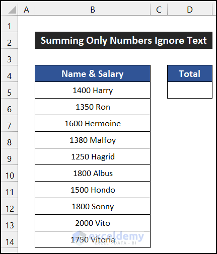
If we manually calculate the sum using a calculator, we get a result of 15,830.

Now, let’s explore six easy methods to achieve the same result programmatically:
Method 1 – Using SUM, LEFT and FIND Functions
In our first method, we will use the SUM, LEFT, and FIND functions to get the sum of only numbers and ignore text in the same cell.
- Select cell D5.
- Enter the following formula in the cell:
=SUM(--LEFT(B5:B14,FIND(" ",B5:B14)))
- Press Enter.
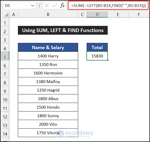
The sum of the numbers will match our manually calculated result. This formula effectively ignores any text within the same cell and only considers the numeric values.
Formula Breakdown for Cell D5:
- FIND(” “,B5:B14): The FIND function searches for the location of ‘Space’ character in all 10 strings. In this case, it returns 5.
- LEFT(B5:B14,FIND(” “,B5:B14)): The LEFT function extracts the numeric values from the strings, with the number of characters equal to the result of the FIND function.
- SUM(–LEFT(B5:B14,FIND(” “,B5:B14))): The SUM function adds up all the extracted numbers, resulting in the final value of 15,830.
Method 2 – Utilizing SUMPRODUCT, LEFT, and FIND Functions
In this method, we’ll use the SUMPRODUCT, LEFT, and FIND functions to achieve the desired result. Follow these steps:
- Select cell D5.
- Enter the following formula in the cell:
=SUMPRODUCT(--LEFT(B5:B14,FIND(" ",B5:B14)))
- Press Enter.
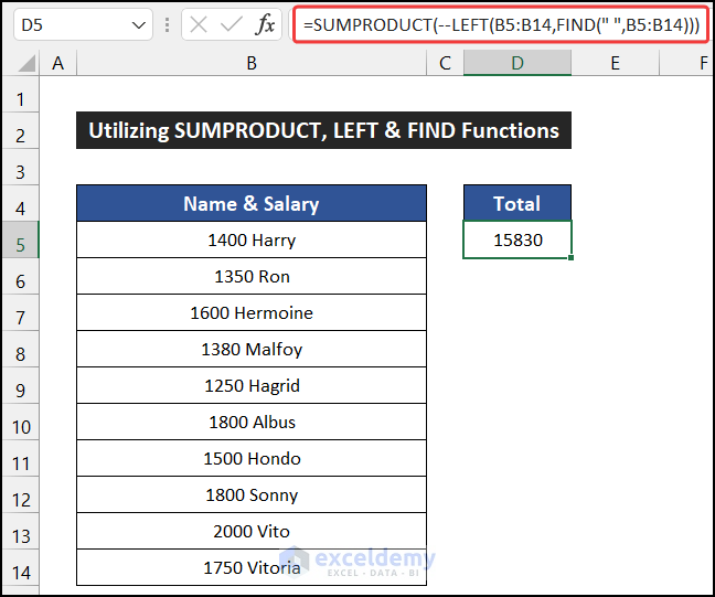
The sum of the numbers will match the manually calculated result. This formula effectively ignores any text within the same cell and considers only the numeric values.
Formula Breakdown for Cell D5:
- FIND(” “,B5:B14): The FIND function searches for the location of a ‘Space’ character in all 10 strings. In this case, it returns 5.
- LEFT(B5:B14,FIND(” “,B5:B14)): The LEFT function extracts the numeric values from the strings, with the number of characters equal to the result of the FIND function.
- SUMPRODUCT(–LEFT(B5:B14,FIND(” “,B5:B14))): Finally, the SUMPRODUCT function adds up all the extracted numbers, resulting in the final value of 15,830.
Method 3 – Using TRIM and IFERROR Functions
In this approach, we’ll utilize the SUM, TRIM, IFERROR, LEFT, and FIND functions to achieve our goal. Follow these steps:
- Select cell D5.
- Enter the following formula in the cell:
=SUM(--TRIM(IFERROR(LEFT(B5:B14,FIND(" ",B5:B14)),0)))
- Press Enter.
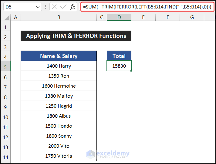
The sum of the numbers will match the manually calculated result. This formula effectively ignores any text within the same cell and considers only the numeric values.
Formula Breakdown for Cell D5
- FIND(” “,B5:B14): The FIND function searches for the location of ‘Space’ characters in all 10 strings. In this case, it returns 5.
- LEFT(B5:B14,FIND(” “,B5:B14)): The LEFT function extracts the numeric values from the strings, with the number of characters equal to the result of the FIND function.
- IFERROR(LEFT(B5:B14,FIND(” “,B5:B14)),0): The IFERROR function checks the result of the LEFT function. If there is a value, the function will show it; otherwise, it will show zero (0).
- TRIM(IFERROR(LEFT(B5:B14,FIND(” “,B5:B14)),0)): The TRIM function eliminates any unnecessary characters from the extracted strings.
- SUM(–TRIM(IFERROR(LEFT(B5:B14,FIND(” “,B5:B14)),0))): Finally, the SUM function adds up all the numbers obtained from the TRIM function, resulting in the final value of 15,830.
Method 4 – Using SUM, IFERROR and RIGHT Functions
In this process, we’ll utilize the SUM, IFERROR, and RIGHT functions to achieve our goal of summing only numbers and ignoring text within the same cell. Note that for this formula to work, the numbers must appear after the text. Let’s break down the steps:
- Select cell D5.
- Enter the following formula in the cell:
=SUM(IFERROR(--RIGHT(B5:B14,4),0))
- Press Enter.
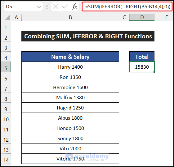
The sum of the numbers will match the manually calculated result. This formula effectively ignores any text within the same cell and considers only the numeric values.
Formula Breakdown for Cell D5:
- RIGHT(B5:B14,4): The RIGHT function extracts the last four digits from each string (representing the salary of the employees).
- IFERROR(–RIGHT(B5:B14,4),0): The IFERROR function checks the result of the RIGHT function. If there is a value, it will be shown; otherwise, zero (0) will be displayed.
- SUM(IFERROR(–RIGHT(B5:B14,4),0)): The SUM function adds up all the numbers obtained from the IFERROR function, resulting in the final value of 15,830.
Method 5 – Summing Only Numbers Based on Categories
In this method, we’ll sum numbers while ignoring text based on specific criteria. To achieve this, we’ll use a combination of functions: SUM, IF, ISNUMBER, VALUE, LEFT, and FIND. Note that we’ll need a different dataset for this approach. Let’s break down the steps:
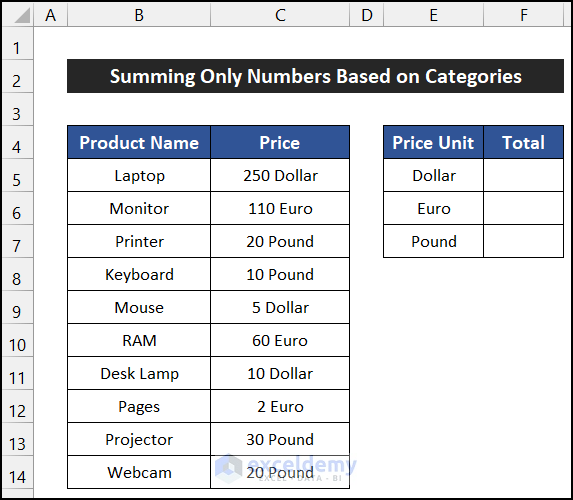
- Select cell F5.
- Enter the following formula in the cell:
=SUM(IF(ISNUMBER(FIND(E5,$B$5:$C$14)),VALUE(LEFT($C$5:$C$14,FIND(E5,$C$5:$C$14)-1)),0))
- Press Enter.
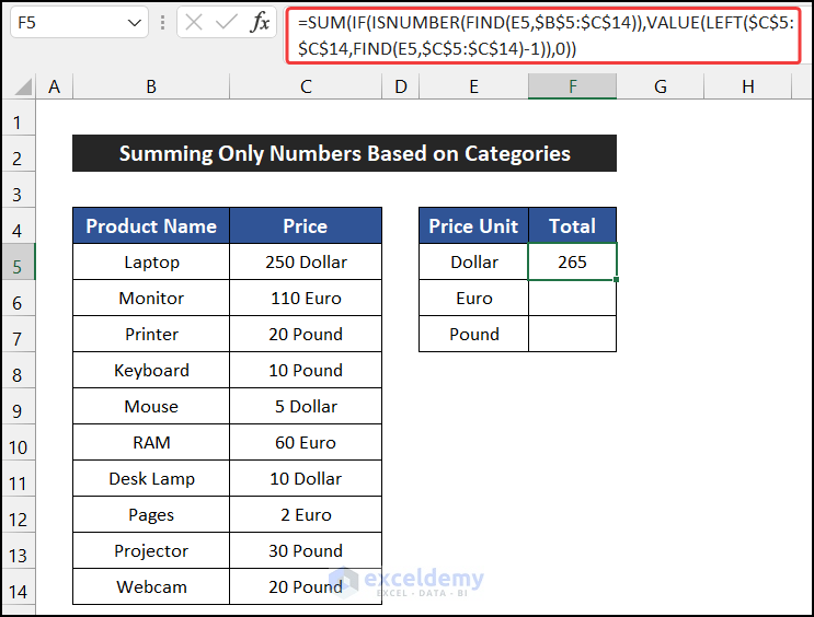
- Double-click on the Fill Handle icon to copy the formula up to cell F7.
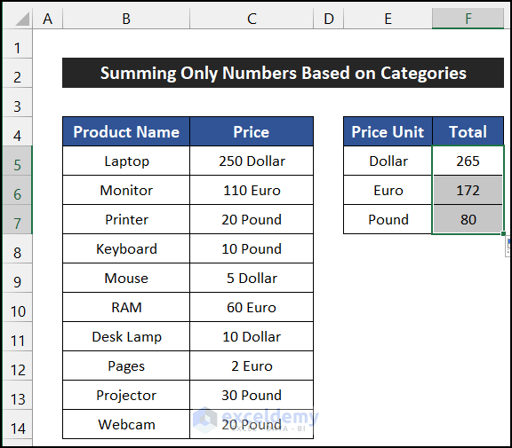
You’ll see the sum of all the numbers based on our three desired categories.
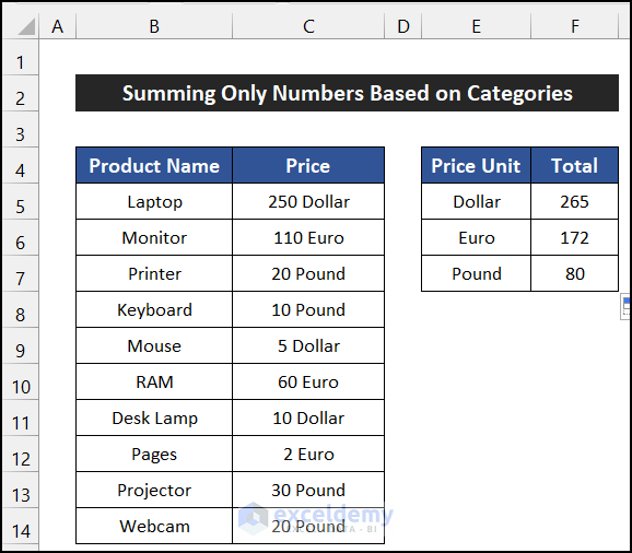
Formula Breakdown for Cell F5
- FIND(E5,$C$5:$C$14): The FIND function checks the value of E5. In this case, the value is 5.
- LEFT($C$5:$C$14,FIND(E5,$C$5:$C$14)-1): The LEFT function extracts the numeric values from the strings. In this cell, it returns 250.
- VALUE(LEFT($C$5:$C$14,FIND(E5,$C$5:$C$14)-1)): The VALUE function converts characters from text to numeric format.
- ISNUMBER(FIND(E5,$B$5:$C$14)): The ISNUMBER function checks the value of the FIND function. Here, it returns TRUE.
- IF(ISNUMBER(FIND(E5,$B$5:$C$14)),VALUE(LEFT($C$5:$C$14,FIND(E5,$C$5:$C$14)-1)),0): This function returns 250.
- SUM(IF(ISNUMBER(FIND(E5,$B$5:$C$14)),VALUE(LEFT($C$5:$C$14,FIND(E5,$C$5:$C$14) -1)),0)): The SUM function adds up all the numbers obtained from the IF function, resulting in the final value of 265.
Method 6 – Embedding VBA Code to Sum Only Numbers and Ignore Text in Excel
If you want to sum only the numeric values in a range of cells while ignoring any text, you can achieve this using VBA (Visual Basic for Applications) code. Follow these steps:
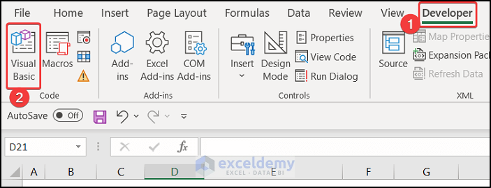
- Go to the Developer tab in Excel.
- Click on Visual Basic to open the Visual Basic Editor.
- If you don’t see the Developer tab, you’ll need to enable the Developer tab.
- Alternatively, you can press Alt + F11 to directly open the editor.
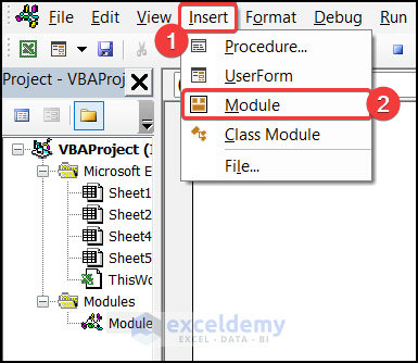
- In the Visual Basic Editor, click on the Insert menu.
- Choose Module to insert a new module.
- In the empty code editor, enter the following VBA function:

Function sum_only_numbers(main_range As Range, Optional str_delim As String = " ") As Double
    Dim data As Variant, long_num As Long
    For Each elem In main_range
      data = Split(elem, str_delim)
      For long_num = LBound(data) To UBound(data) Step 1
        sum_only_numbers = sum_only_numbers + Val(data(long_num))
      Next long_num
    Next elem
End Function- Press Ctrl + S to save the code.
- Close the Visual Basic Editor.
- Select the cell where you want to display the sum (e.g., cell D5).
- Enter the following formula:
=sum_only_numbers(B5:B14)
- Press Enter.
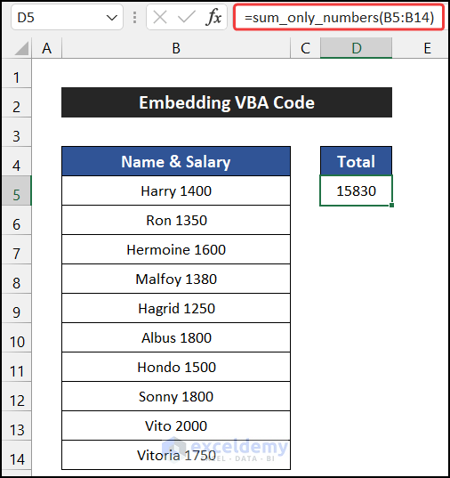
You’ll now see the sum of all the numeric values in the specified range (B5:B14), excluding any text. This approach successfully allows you to sum only numbers and ignore text within the same cell in Excel.
Download Practice Workbook
You can download the practice workbook from here:
Related Articles
- How to Sum If Cell Contains Text in Another Cell in Excel
- How to Sum Names in Excel
- How to Assign Value to Text and Sum in Excel
- How to Sum Text Values Like Numbers in Excel
<< Go Back to Excel Sum If Cell Contains Text | Excel SUMIF Function | Excel Functions | Learn Excel
Get FREE Advanced Excel Exercises with Solutions!

