Method 1 – Using the Percent Style Button in the Number Group
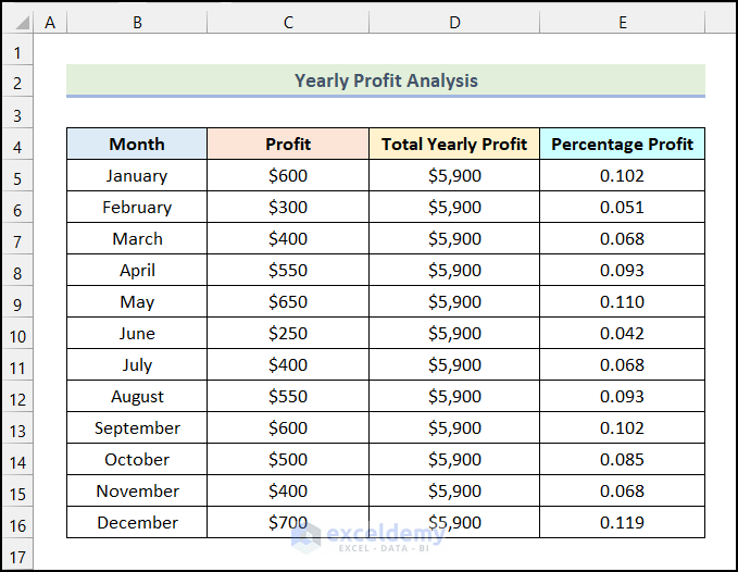
A company needs to determine the Profit Percentage for 12 months. They have calculated the amount of profits which are displayed as decimals in the column Percentage Profit. To convert the numbers into percentages:
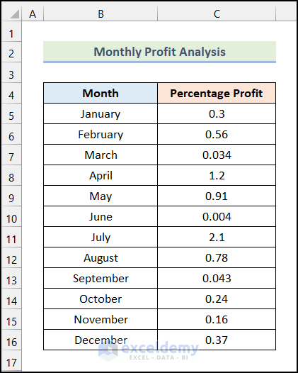
Steps:
- Select all cells containing decimals and numbers in the Percentage Profit column.
- In the Home tab, click % (Percent Style) in Number.
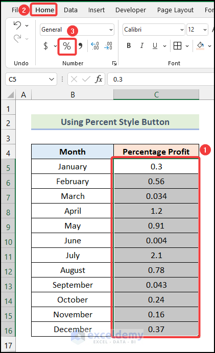
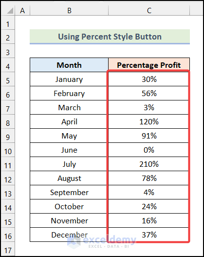
Percentages are displayed.
Method 2 – Utilizing the Custom Number Format Option
To add Percentage Symbols beside all values without changing the data:
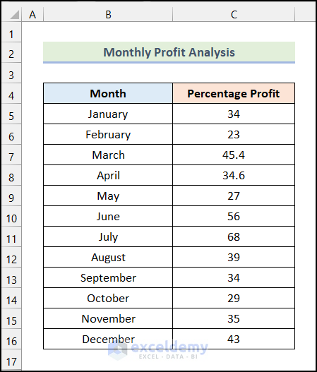
Steps:
- Select all the cells in the Percentage Profit column.
- In the Home tab, select Number and click Number Format.
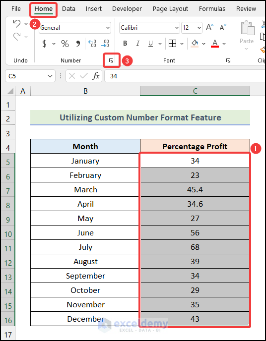
- In Format Cells will appear, select Custom in Number.
- Click General in Type.
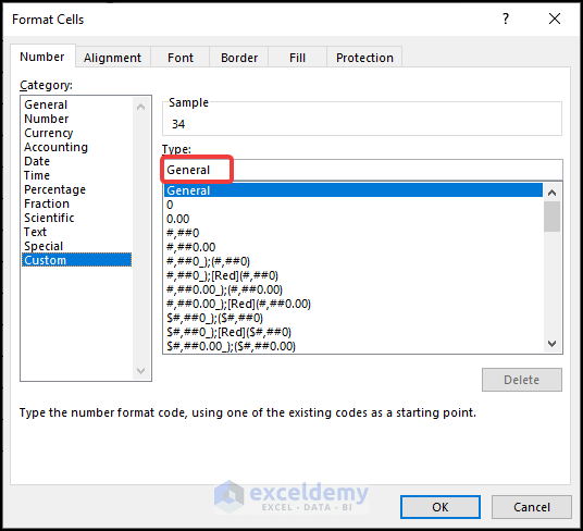
Note: You can press CTRL + 1 to open the Format Cells dialog box.
- Enter the following format code in Type.
0\%- Click OK.
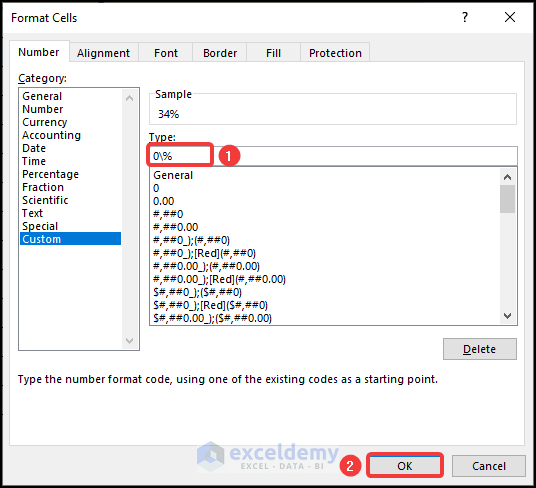
All values are in percentage format.
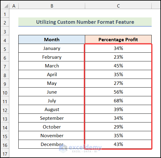
To add decimal places:
- Select the cells in the Percentage Profit column and go to the Home tab.
- Click Number Format in Number.
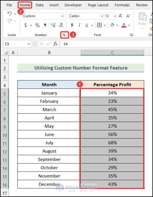
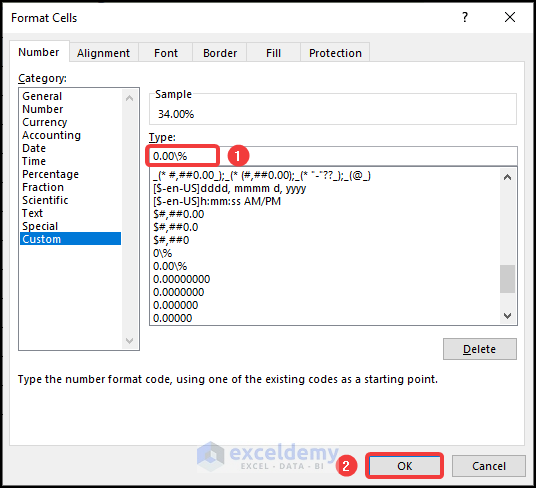
- Replace 0\% with 0.00\% to add 2 decimal places.
- Click OK or press ENTER.
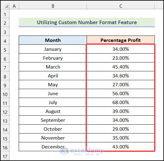
You will see percentage values with 2 decimal places.
Read More: How to Divide a Value to Get a Percentage in Excel
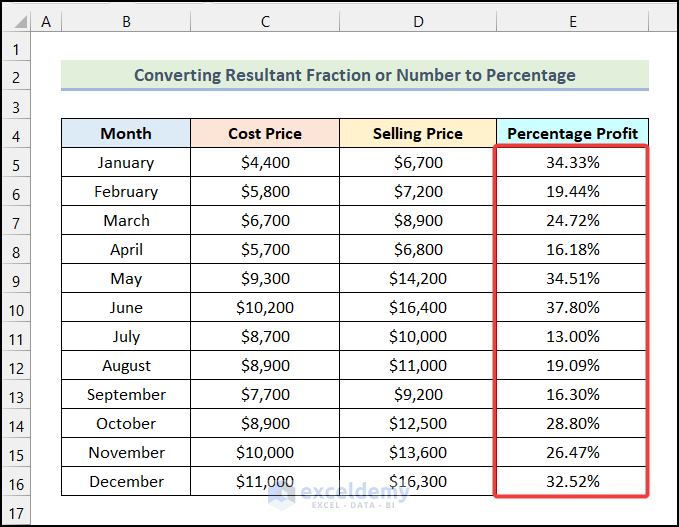
Method 3 – Converting a Resultant Fraction or Number to a Percentage in Excel
To find the Percentage Profits:
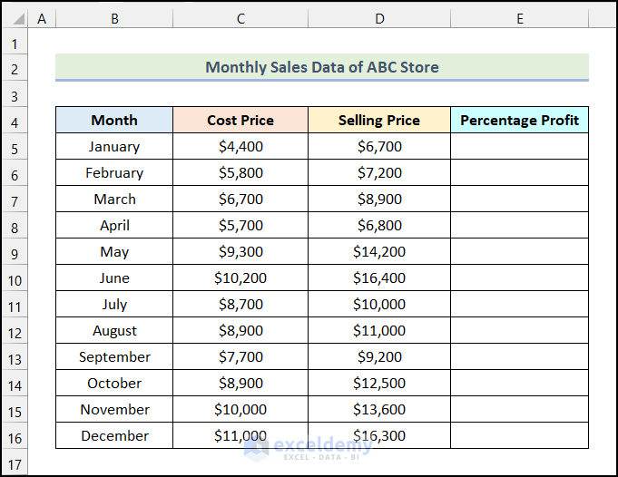
Steps:
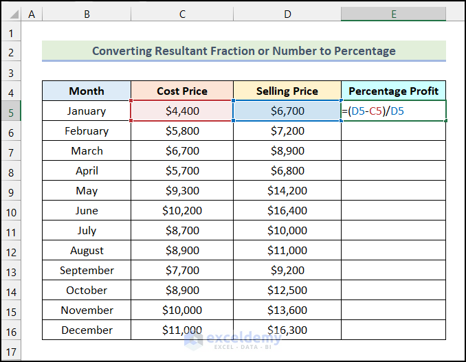
- Use the following formula in E5.
=(D5-C5)/D5D5 refers to the cell in the Selling Price column, and C5 indicates the cell in the Cost Price column.
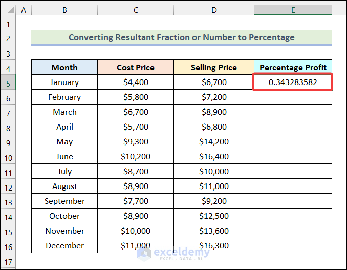
- Press ENTER.
This is the output.
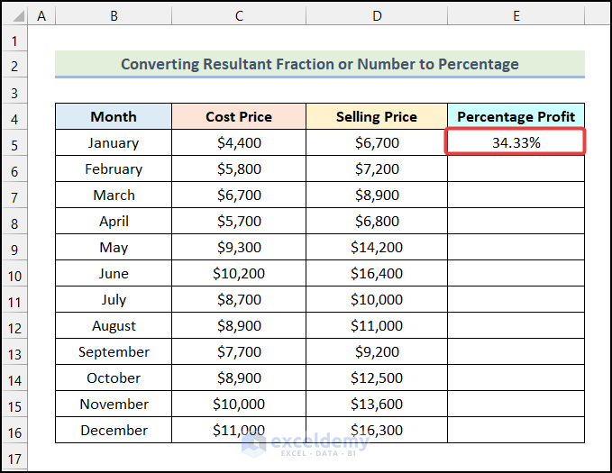
- Follow the steps in the 2nd method to obtain the following output in E5.
- In E5, point your mouse cursor to the right bottom corner, and you’ll find a ‘+’ icon: the Fill Handle.
- Drag down the Fill Handle to see the result in the other cells.
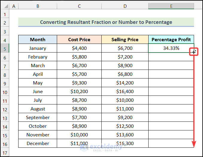
The Percentage Profit for all Months is displayed.
How to Convert a Number to Percentage in an Excel Pivot Table
The dataset showcases the Yearly Profit Analysis of a company. To convert numbers in the Percentage Profit column into percentage:
Steps:
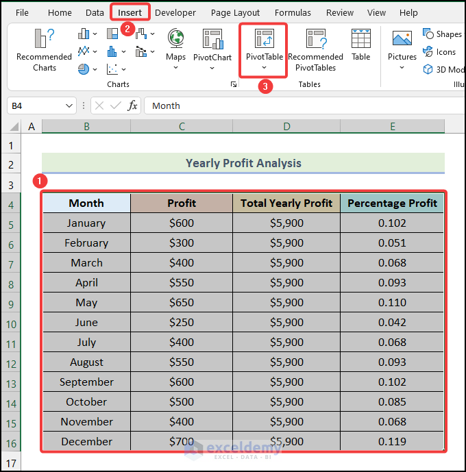
- Select the dataset and go to the Insert tab.
- Select Pivot Table in Tables.
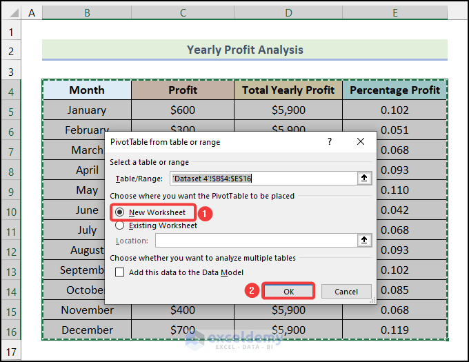
- Choose New Worksheet in the dialog box PivotTable from table or range.
- Click OK.
The Pivot Table Fields dialog box will be displayed.
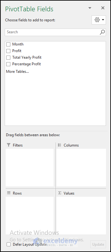
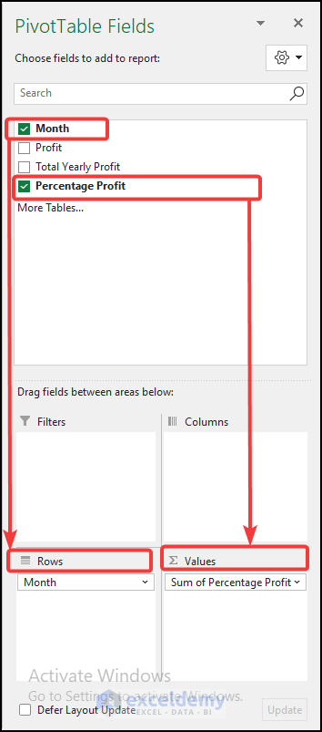
- Select Month and drag it into Rows.
- Select Percentage Profit and drag it into Values.
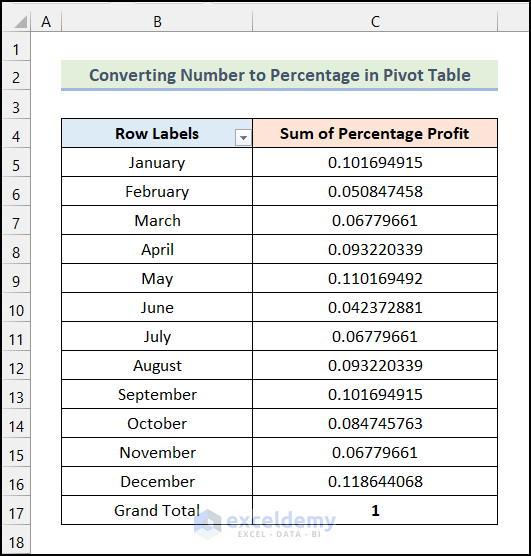
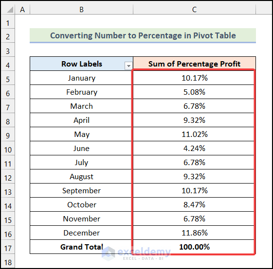
This is the output.
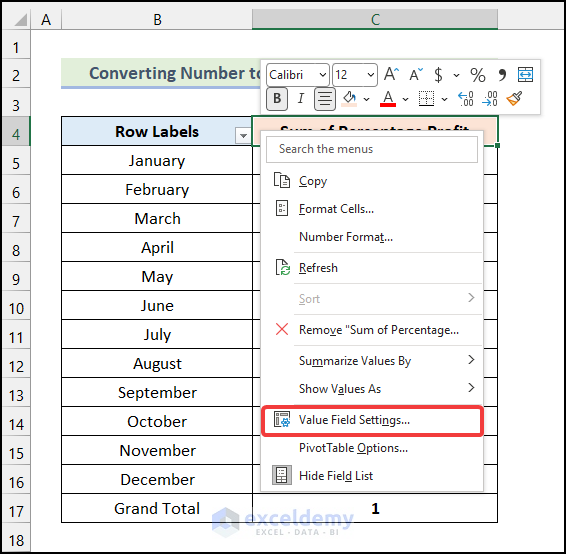
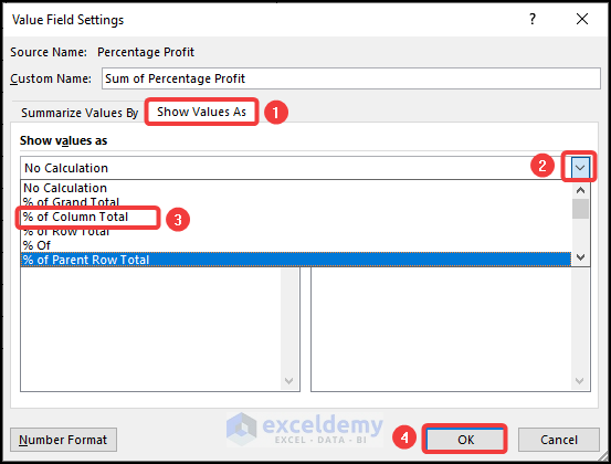
- Right-click C4 and click Value Field Settings.
- In the Value Field Settings dialog box, go to Show Values As.
- Click the drop-down icon.
- Choose % of Column Total.
- Click OK.
This is the final output.
Read More: How to Do Sum of Percentages in Excel
How to Convert Number to Percentage in Excel Charts
Steps:
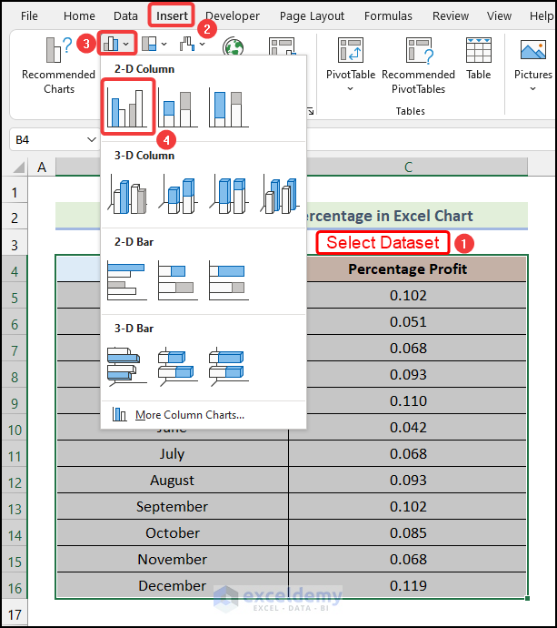
- Select the dataset and go to the Insert tab.
- Select Insert Column or Bar Chart in Charts.
- Choose Clustered Column.
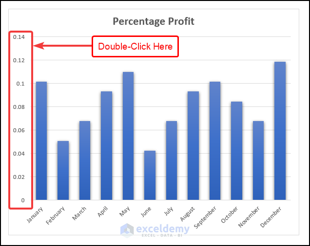
The following chart will be displayed.
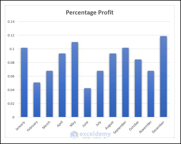
- Double-click the vertical axis of the chart.
The Format Axis dialog box will be displayed.
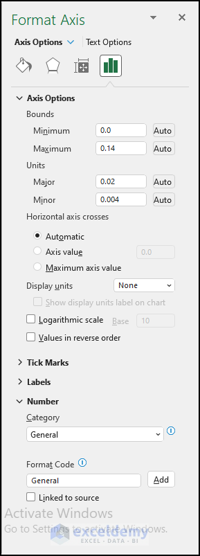
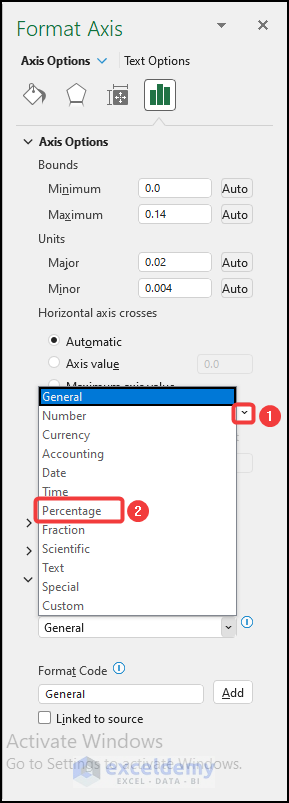
- In Format Axis, select Number and click the drop-down icon under Category.
- Choose Percentage.
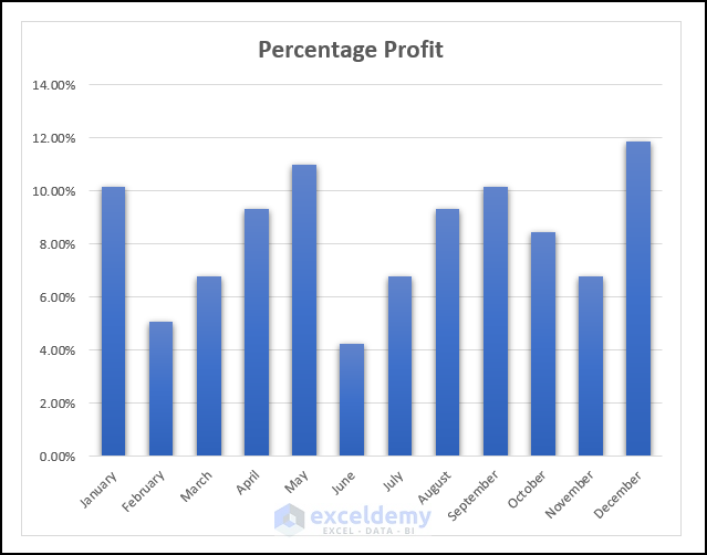
This is the output.
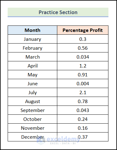
Practice Section
Practice here.
Download Practice Workbook
Download the worksheet here.
Related Articles
- How to Calculate Percentage of Total in Excel
- Convert Number to Percentage Without Multiplying by 100 in Excel
- How to Calculate Reverse Percentage in Excel
- How to Find the Percentage of Two Numbers in Excel
- How to Convert Percentage to Number in Excel
- How to Convert Percentage to Whole Number in Excel
- How to Show One Number as a Percentage of Another in Excel
- How to Add a Percentage to a Number in Excel
- Make an Excel Spreadsheet Automatically Calculate Percentage
<<Go Back to Calculating Percentages in Excel | How to Calculate in Excel | Learn Excel
Get FREE Advanced Excel Exercises with Solutions!

