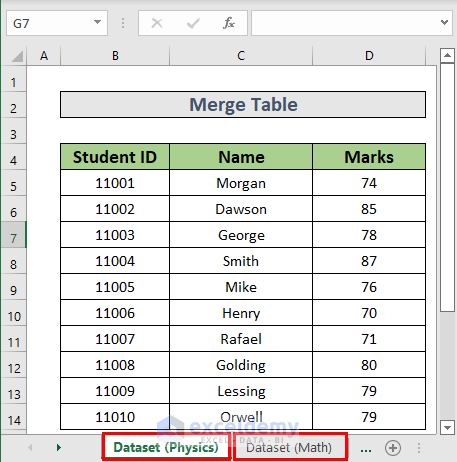
The two sample sheets contain data of student names and marks obtained for Physics and Math.
Method 1 – Apply the VLOOKUP Function to Merge Tables from Different Sheets
Steps:
- Go to E5 and insert the following formula
=VLOOKUP(B5,'Dataset (Math)'!$B$5:$D$14,3,FALSE)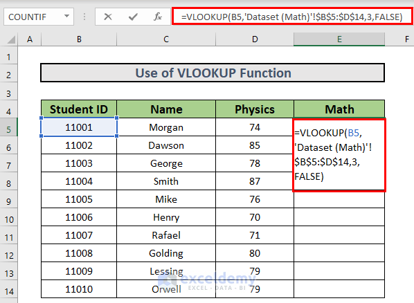
Formula Explanation:
- B5 is the lookup_value.
- Excelwill look for the value in B5 (11001) in the range B5:D14 from the Dataset (Math)
- 3states that Excel will find 3rd column from the range.
- FALSEis for Exact Match.
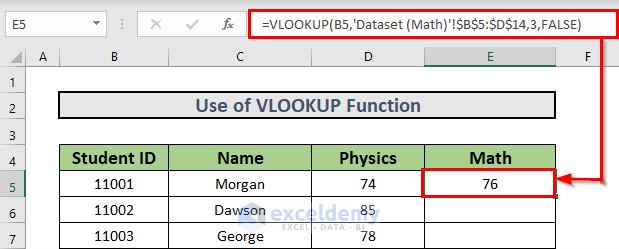
- Press ENTERto get the output.
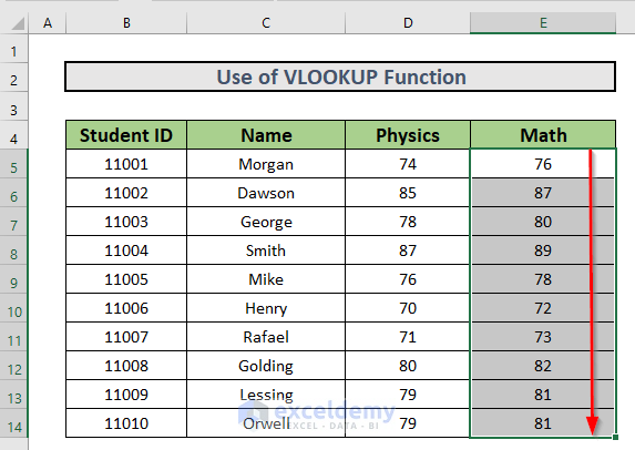
- Use the Fill Handle to AutoFill up to E14.
Read More: How to Merge Two Tables in Excel Using VLOOKUP
Method 2 – Use a Combination of INDEX and MATCH Functions to Merge Tables
Steps:
- Go to E5 and insert the following formula.
=INDEX('Dataset (Math)'!$D$5:$D$14,MATCH('Dataset (Math)'!D5,'Dataset (Math)'!$D$5:$D$14,0))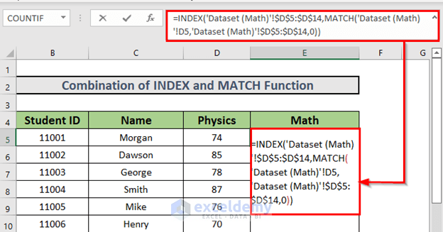
Formula Breakdown:
- MATCH(‘Dataset (Math)’!D5,’Dataset (Math)’!$D$5:$D$14,0)
- Output: 1
- INDEX(‘Dataset (Math)’!$D$5:$D$14,MATCH(‘Dataset (Math)’!D5,’Dataset (Math)’!$D$5:$D$14,0)) → This becomes,
- INDEX(‘Dataset (Math)’!$D$5:$D$14,1
- Output: 76
- Press ENTER to get the output.
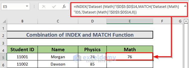
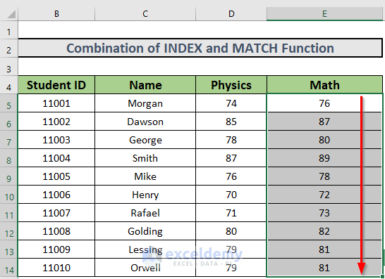
- AutoFill up to E14.
Method 3 – Merge Tables from Different Sheets Using Consolidate Feature
Steps:
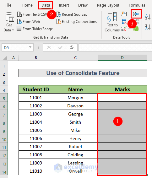
- Select D5:D14.
- Go to Data.
- Select the Consolidate feature (see image).
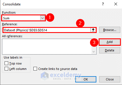
- Choose the function Sum.
- Select the reference for the marks of Physics.
- Click Add.
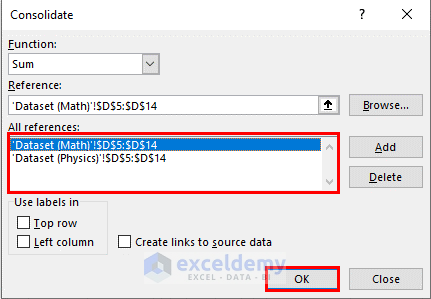
- Add the marks for Math.
- Click OK.
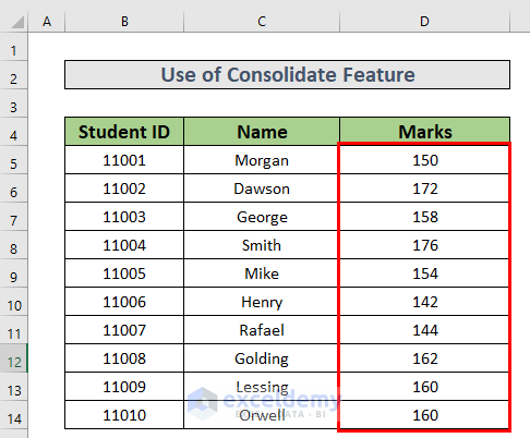
- Excel will add the marks.
Read More: How to Merge Two Tables in Excel
Method 4 – Use PowerQuery to Merge Tables from Different Sheets
Steps:
- Convert data ranges to tables.
- Select B4:D14.
- Press CTRL+T.
- The Create Table box will appear.
- Check My table has headers.
- Click OK.
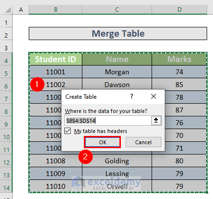
- Excel will create a table.
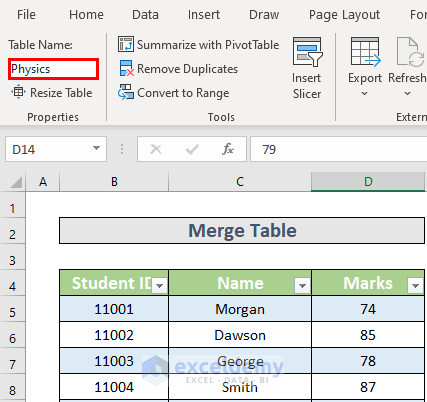
- Rename the table as Physics.
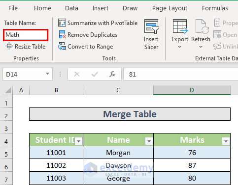
- Create a second table and name it Math.
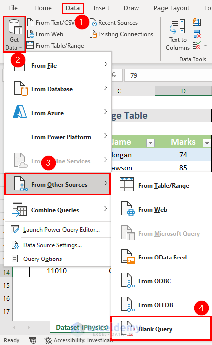
- Go to the Data
- Select Get Data.
- Choose From Other Sources.
- Select Blank Query.
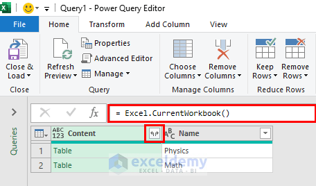
- The Power Query Editor will appear.
- Insert the following formula:
=Excel.CurrentWorkbook()- Press ENTER.
- Select the icon shown in the image.
- Uncheck the ‘Use original column name as prefix’ box.
- Click OK.
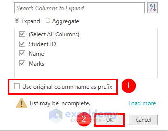
- Excel will merge the tables.
- Click Close & Load.
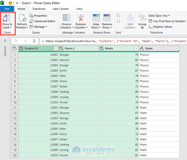
- Excel will load the combination in a new worksheet.
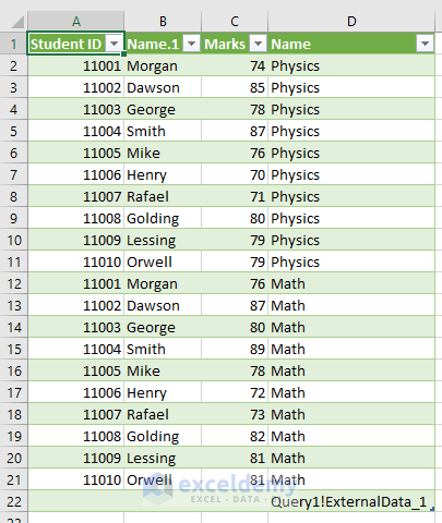
- A new row Query1!ExternalData_1 appears. To remove this, select the drop-down.
- Uncheck the box for Query1!ExternalData_1.
- Click OK.
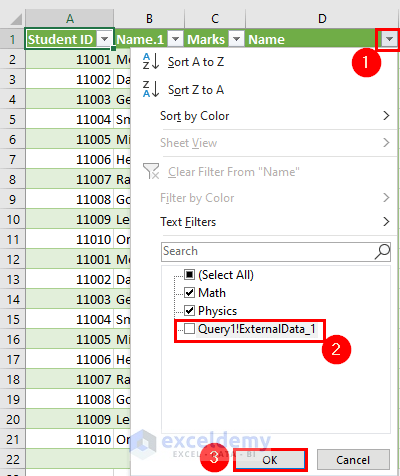
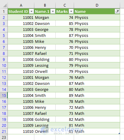
- The tables merged. The final output will be as shown in the image.
Method 5 – Use VBA Code to Merge Tables from Different Sheets
Steps:
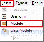
- Press ALT+F11 to open the Visual Basic Editor.

- Go to Insert
- Select Module.
- A new module will appear. Insert the following code.
Sub MergeTable()
Worksheets("VBA").Range("B4:D14").Value = Worksheets("Dataset (Physics)").Range("B4:D14").Value
Worksheets("VBA").Range("E4:E14").Value = Worksheets("Dataset (Math)").Range("D4:D14").Value
End Sub
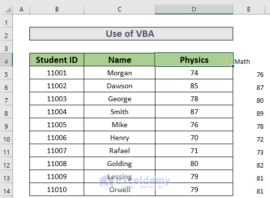
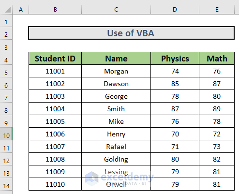
- Press F5 to run the code. Excel will merge the columns from those tables.
- Format as required.
Download the Practice Workbook
<< Go Back to Merge Tables in Excel | Merge in Excel | Learn Excel
Get FREE Advanced Excel Exercises with Solutions!

