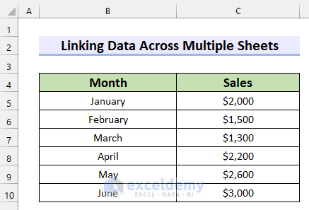
How to Link Excel Data Across Multiple Sheets (7 Easy Ways)

Let’s consider the following dataset to explain this article, which contains the Month and Sales columns.

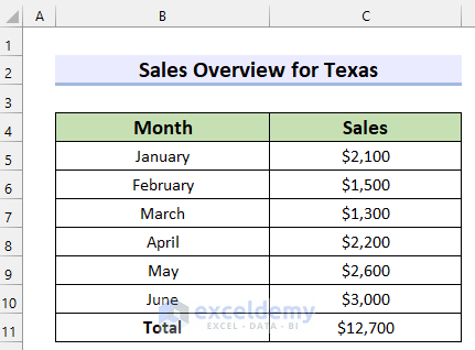
For this article, we have 3 sheets. These sheets contain the Sales Overview of a particular State. The first sheet contains the Sales Overview for Texas.

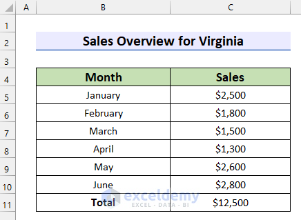
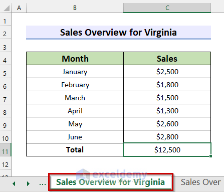
The second sheet contains the Sales Overview for Virginia.

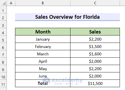
And, the third sheet contains the Sales Overview for Florida.

Method 1 – Using Paste Special Option to Link Excel Data Across Multiple Sheets

Here, we will link the Total Sales of every sheet to a new sheet to show the Total Sales for every State together.

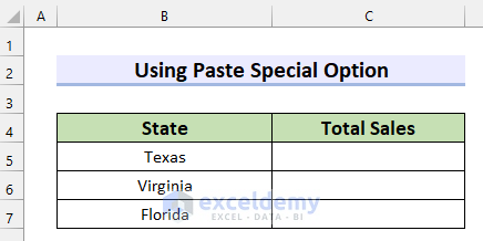
Steps:

Select the cell from where you want to link the data. We selected cell C11 because it contains the Total Sales for Texas.
Copy the cell by pressing Ctrl + C.

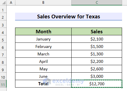
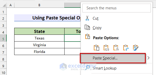
Select the cell where you want to link the data. We selected cell C5 from the sheet named Sales Overview for Texas.
Right-click on the cell.
Select Paste Special.

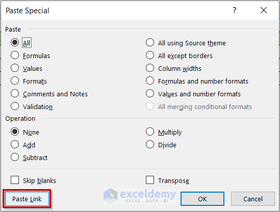
A dialog box named Paste Special will appear. Select Paste Link.
Click on OK.

This pastes the data with a link. If you change the source data it will be updated automatically.

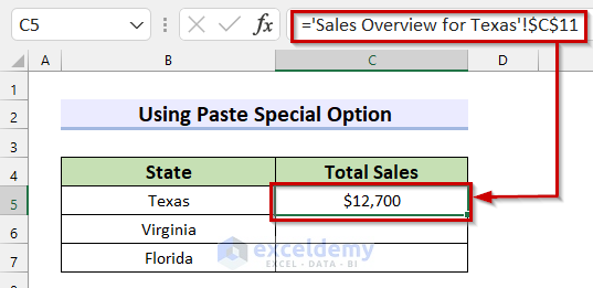
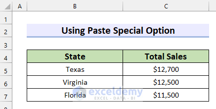
Copy the other values using the Paste Special option in the same way.

Read More: How to Link Two Sheets in Excel

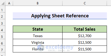
Method 2 – Applying Sheet Reference to Link Data Across Multiple Sheets in Excel

Steps:

Select the cell where you want to link the data. We selected cell C5.
Copy the following formula into it:

='Sales Overview for Texas'!C11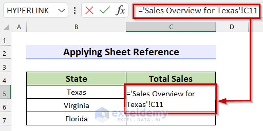

Here, I have used the cell sheet reference to link the data. This formula will return the data that is in cell C11 of the sheet named Sales Overview for Texas.

Press Enter and you will get your linked data.

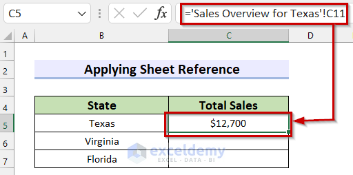
Repeat the process for the other sheets.

Method 3 – Using Link Option to Insert Hyperlink

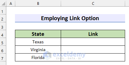
Let’s put the hyperlinks to the Total Sales for every State in the following table.

Steps:

Select the cell where you want to insert the link. We selected cell C5.
Right-click on the cell.
Select Link.

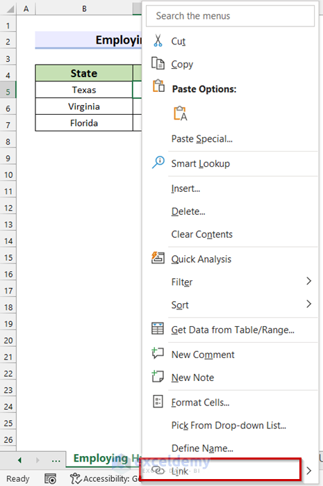
A dialog box named Insert Hyperlink will appear.
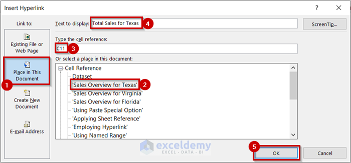
Select Place in This Document from the Link to section.
Choose the sheet that has the data you want to link. We used the sheet named Sales Overview for Texas.
Select the cell that carries the data. We selected cell C11 because this cell carries the Total Sales.
Type the text you want to display in the cell. We put Total Sales for Texas.
Select OK to insert the link.

You will see the link to that particular cell has been inserted into your selected cell.

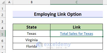
Repeat for other links in the same way.

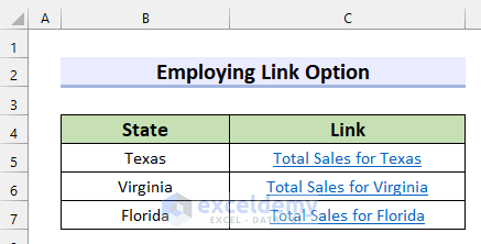
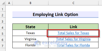
Now, you can click on any link to see that particular data. Here, we clicked on Total Sales for Texas.

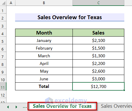
You can see that the link leads to the linked cell of that particular sheet that carries the Total Sales for Texas.

Method 4 – Applying HYPERLINK Function to Link Data

Steps:

Select the cell where you want to insert the link, such as C5.
Copy the following formula into it:

=HYPERLINK("#'Sales Overview for Texas'!C11","Total Sales for Texas")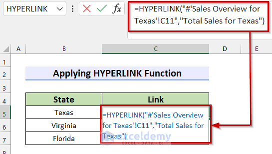

Now, in the HYPERLINK function, we selected “#’Sales Overview for Texas’!C11” as link_location, and “Total Sales for Texas” as friendly_name. The function will return a link that will directly lead to the selected location which is cell C11 of the sheet named Sales Overview for Texas.

Press Enter, and you will get the link.

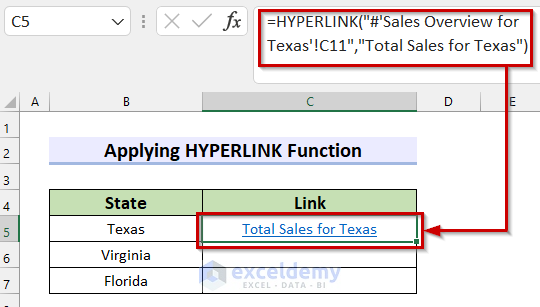
Insert the other links in the same way.

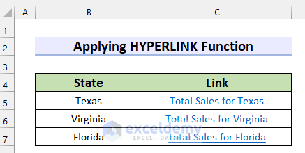
After that, you can select any link and then click on that link to see that particular data. Here, we clicked on Total Sales for Virginia.

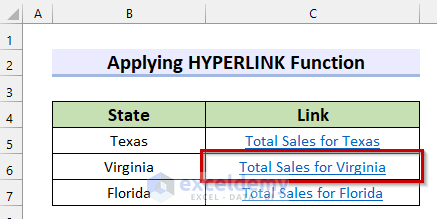
You can see that the link leads to the linked cell of that particular sheet that carries the Total Sales for Virginia.

Method 5 – Using Named Range to Link Data Across Multiple Sheets

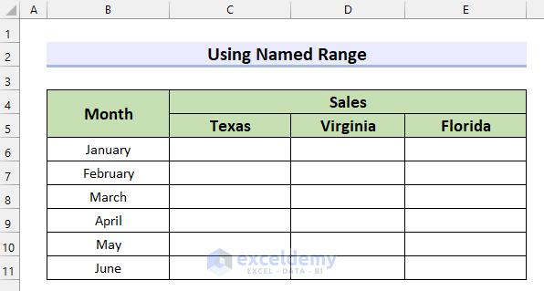
Here’s a dataset with the Sales for every Month for each State in the same sheet, which we will fill by linking the data.

Steps:

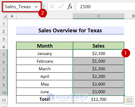
Select the data range you want to link.
Give this range a name. We named the first one from the Texas worksheet as Sales_Texas. This name will always refer to this range.

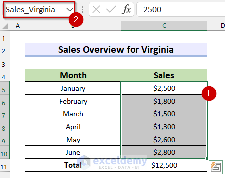
Repeat for other sheets and names. For the sheet with sales in Virginia, we used Sales_Virginia.

For Florida sales, we put Sales_Florida.

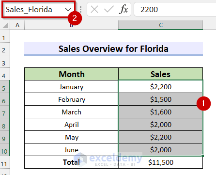
Select the cell from where you want to start the linked range. We selected cell C6.
In that cell, input the following formula:

=Sales_Texas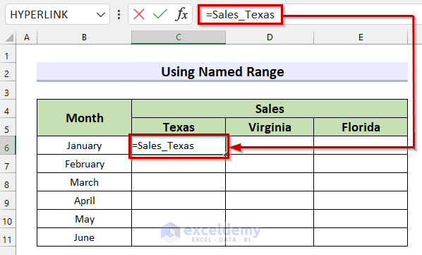

The formula will return the data range named Sales_Texas.

Press Enter to get the linked range.

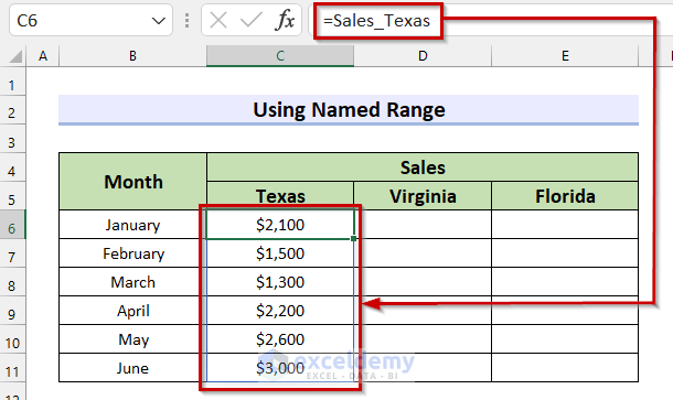
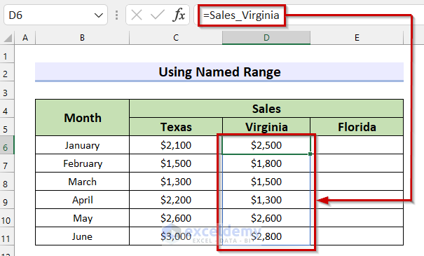
Select the next cell to link data, C6.
Input the following formula:

=Sales_Virginia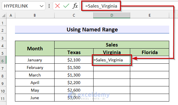

Here, the formula will return the data range named Sales_Virginia.

Press Enter and you will get the linked range.

Select cell E6.
Copy the following into it:

=Sales_Florida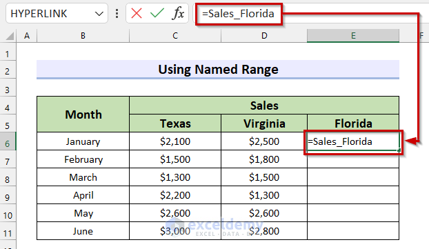

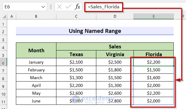
Here, the formula will return the data range named Sales_Florida.

Press Enter and you will fill the table.

Method 6 – Use of 3D Formula to Link Excel Data Across Multiple Sheets

Let’s add the Sales for every Month from three different sheets and show them on another sheet. But, to use this type of formula you have to have data in the same cell on every sheet.

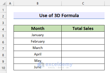
Steps:

Select the cell where you want to link the data. We selected cell C5.
Input the following formula:

=SUM('Sales Overview for Texas:Sales Overview for Florida'!C5)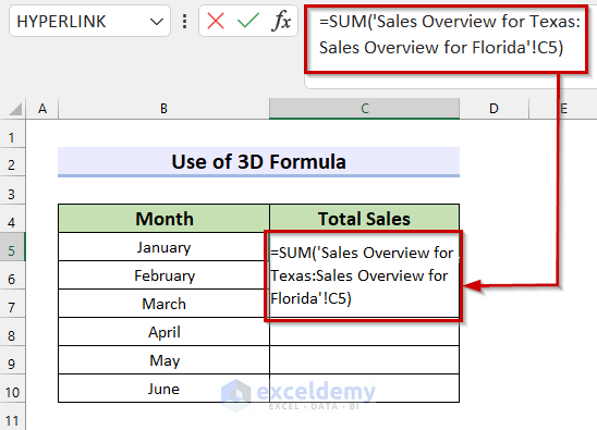

To write this formula manually, in the SUM function select the cell that contains the data you want to sum from the first sheet then press and hold the SHIFT key while selecting the last sheet. This formula will return the summation of the values in cell C5 from the sheet named Sales Overview for Texas to the sheet named Sales Overview for Florida.

Press Enter to get the result.

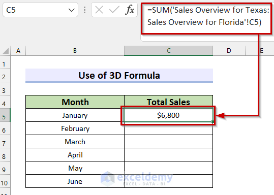
Drag the Fill Handle to copy the formula.

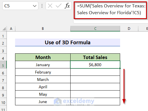
Excel has copied the formula to all the cells.

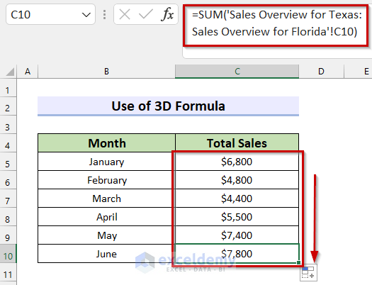
Method 7 – Applying Consolidate Command to Link Data Across Multiple Sheets

Steps:

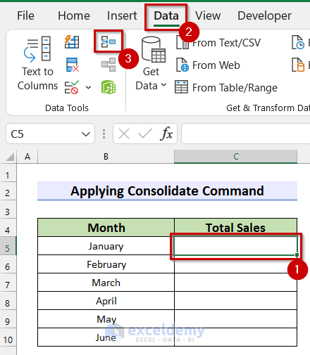
Select the cell from where you want to link your data range. Here, we selected cell C5.
Go to the Data tab.
Select Consolidate.

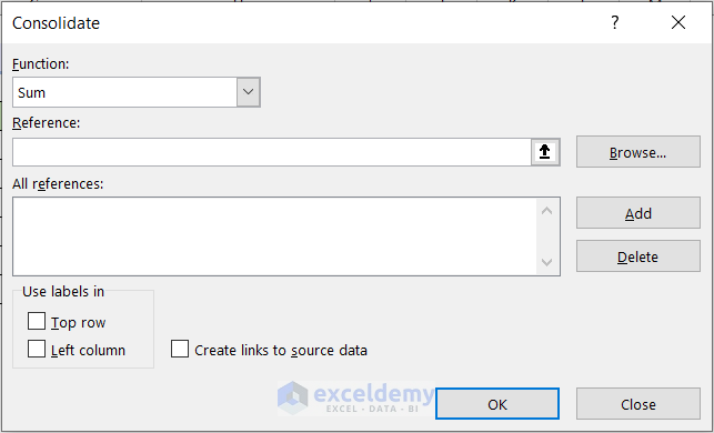
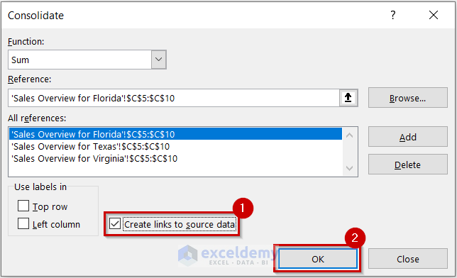
A dialog box named Consolidate will appear.

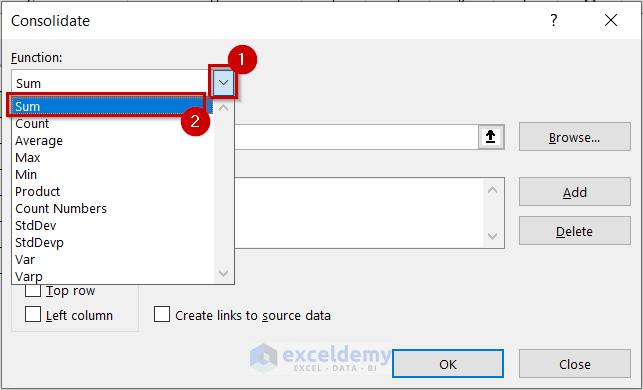
Select the drop-down option for Function.
Choose the function you want. We’ll use the Sum function.

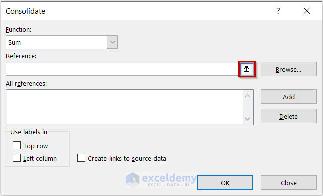
Select the up arrow in the Reference box to select the Reference.

Select the range for Reference.
Click on the arrow at the end of the box to add the Reference.

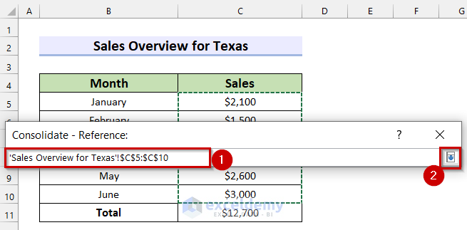
Select Add.

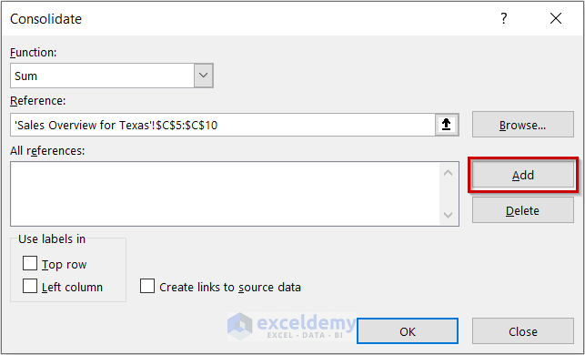
Here, you will see your selected range is added to the All references.

Repeat to select the second Reference.

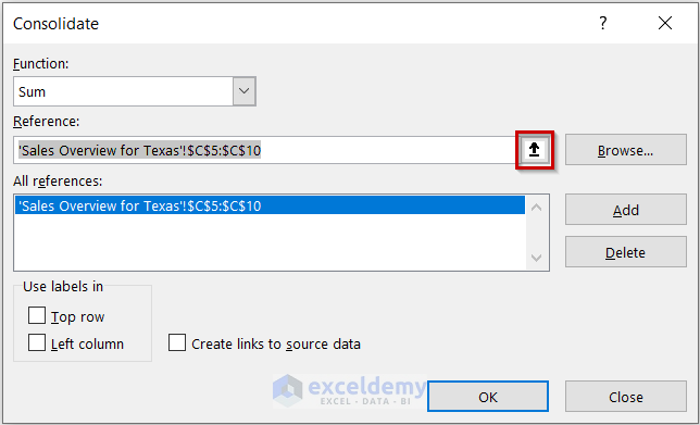
Select the next range for Reference.
Add the Reference with the arrow button at the end of the box.

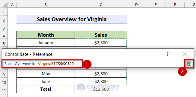
Select Add.

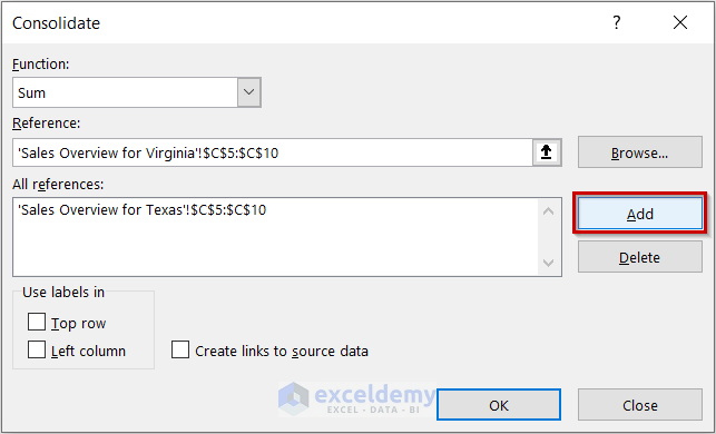
Now, you will see your selected second range is added to the All references.

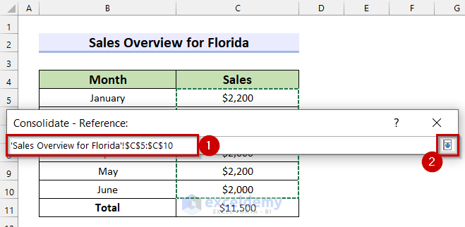
Repeat for the third Reference.

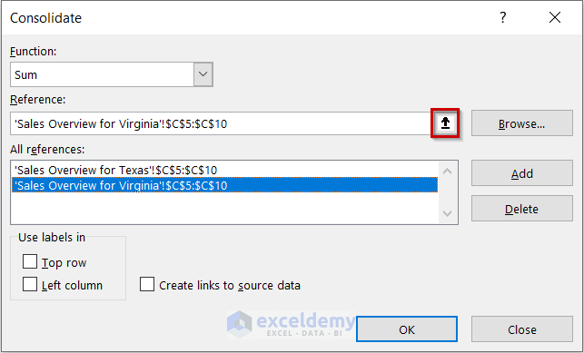
Select the range for the Reference and confirm.

Click on Add.

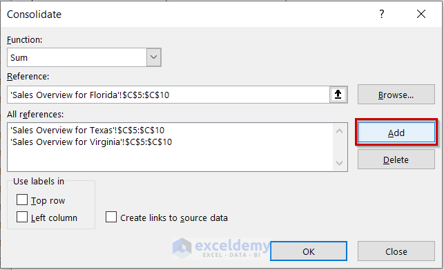
Here, you will see all the selected ranges are added to the All references.

Check the Create links to source data option.
Select OK.

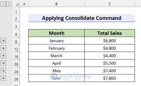
You have created your consolidated data that are linked to the source data.

Things to Remember

Whenever using the 3D formula it should be kept in mind that all the sheets must contain the value in the same cells.
If you are using the Consolidate command to link the range then the data must be of the same type and they have to be in the same layout.