Method 1 – Using the SUBSTITUTE Function to SUM Cells with Text and Numbers
The SUBSTITUTE function can separate the text from the numeric values.
The syntax of the SUBSTITUTE function is as follows:
=SUBSTITUTE (text, old_text, new_text, [instance])text: The cell or cells to modify.
old_text: The old text to replace.
new_text: The new text to replace with.
instance [Optional]: The instance to replace. By default, all instances will be replaced.
You can learn about this function in detail by reading this documentation from Microsoft.
Importantly, the syntax of the SUM function is as follows:
=SUM(number1, [number2] ,…)We need to calculate the Total Weight of the Products in cell D10 by adding the individual weights of Column D.
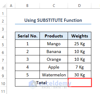
- Insert the following formula in the D10 cell:
=SUM(SUBSTITUTE(D5:D9, " Kg", "")+0)D5:D9 refers to the Weights of Products.
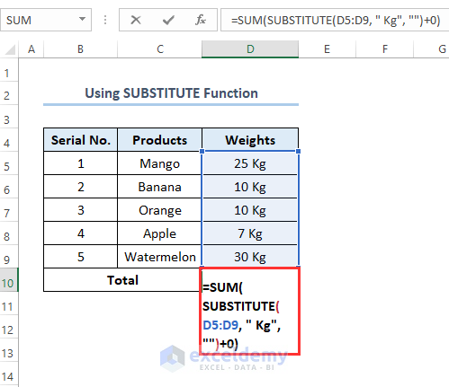
- Press Enter.
- We’ll get the output.
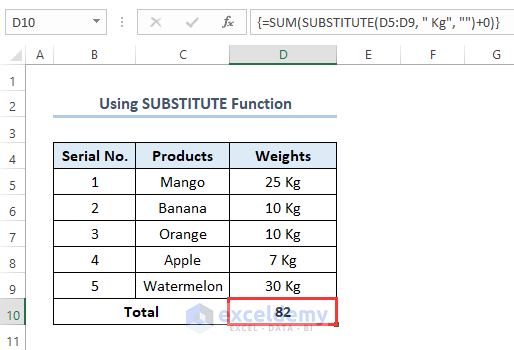
Formula Breakdown:
{=SUM(SUBSTITUTE(D9:D13, ” Kg”, “”)+0)}
- SUM(SUBSTITUTE(“25 Kg, 10 Kg, 10 Kg, 7 Kg, 30, Kg”, ” Kg”, “”)+0)
- SUM(“25, 10, 10, 7, 30” +0)
- SUM(25, 10, 10, 7, 30)
- 82
Read More: All the Easy Ways to Add up (Sum) a column in Excel
Similar Readings
- Add Rows in Excel with Formula (5 ways)
- How to Assign Value to Text and Sum in Excel (2 Easy Methods)
- [Fixed!] Excel SUM Formula Is Not Working and Returns 0 (3 Solutions)
- Use SUMIF with Text in Excel (9 Easy Ways)
- How to Sum Multiple Rows and Columns in Excel
Method 2 – Utilizing the LEFT and FIND Functions
The syntax of the FIND function is as follows:
=FIND (find_text, within_text, [start_num])find_text: The text which is to find.
within_text: The text which is to search within.
start_num [Optional]: The starting position of the search. By default, start_num=1. The first character in within_text is character number 1.
You can learn about this function in detail by reading this documentation from Microsoft.
The syntax of the LEFT function is as follows:
=LEFT (text, [num_chars])text: The text string to extract the characters from.
num_chars [Optional]: The number of characters to extract. It starts from the left. By default, num_chars=1.
The syntax of the VALUE function is as follows:
=VALUE (text)text: The text which is to convert into numbers.
You can check out the first method’s the SUM function section for understanding the function. It is explained there.
We also need to calculate the Total Weight of the Products in cell D10 by adding the individual weights of column D.
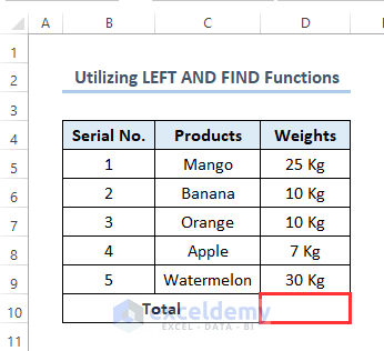
- Use the following formula in the D10 cell:
=SUM(VALUE(LEFT(D5:D9,FIND(" ",D5:D9)-1)))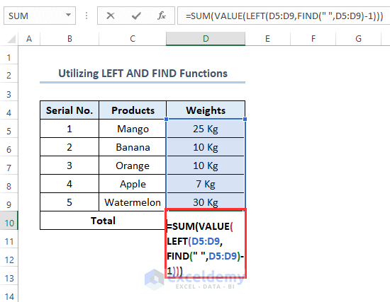
- Press Enter to get the output.
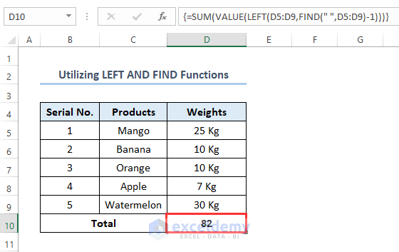
Formula Breakdown:
{=SUM(VALUE(LEFT(D9:D13,FIND(” “,D9:D13)-1)))}
- SUM(VALUE(LEFT(D9:D13,FIND(” “,”25 Kg, 10 Kg, 10 Kg, 7 Kg, 30Kg”)-1)))
- SUM(VALUE(LEFT(D9:D13,(3, 3, 3, 2, 3)-1)))
- SUM(VALUE(LEFT(D9:D13,(2, 2, 2, 1, 1))))
- SUM(VALUE(LEFT(“25 Kg, 10 Kg, 10 Kg, 7 Kg, 30Kg”,(2, 2, 2, 1, 1))))
- SUM(VALUE(25, 10, 10, 7, 30))
- SUM(25, 10, 10, 7, 30)
- 82
Read More: How to Add Numbers in Excel (2 Easy Ways)
Method 3 – Applying a Combined Formula
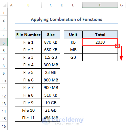
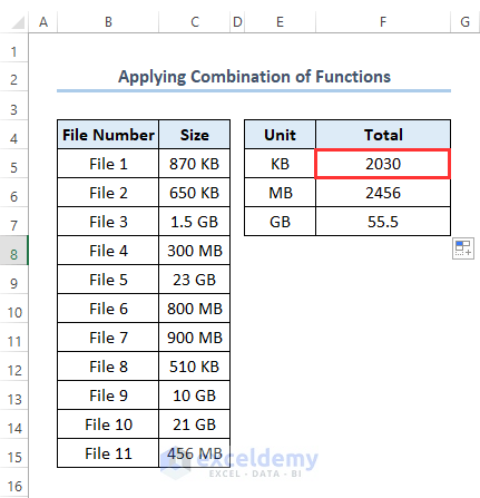
Suppose we have the dataset below which has column headers as File Number and Size in Columns B and C, respectively. The sizes of the files are in three different units: KB, MB, and GB. We need to calculate the total of KB, MB, and GB in Column F with the column header of Total.
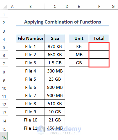
- Use the following formula in the F5 cell:
=SUM(IF(ISNUMBER(FIND(E5,$C$5:$C$15)),
VALUE(LEFT($C$5:$C$15,FIND(E5,$C$5:$C$15)-1)),0))
C5:C15 refers to the cells of column header Size and E5 refers to KB in the column header Unit.
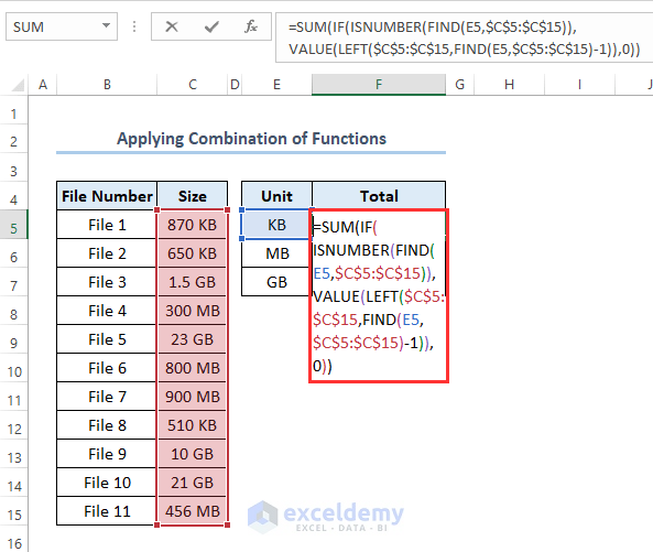
- Press Enter.
- Use the Fill Handle by dragging down the cursor while holding the right-bottom corner of the F5 cell.
- We will get the total of KB, MB, and GB as outputs.
Read More: How to Sum Selected Cells in Excel (4 Easy Methods)
How to SUM Cells with Text via COUNTIF in Excel
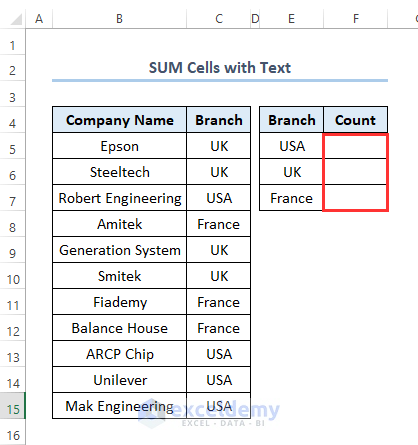
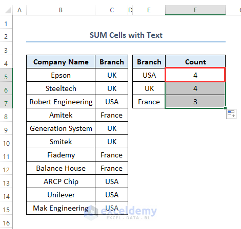
Suppose we have the following dataset with column headers as Company Name and Branch. We need to find out the sum of common branches in Column F with the column header as Count.
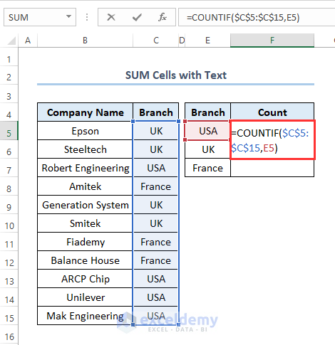
- Use the following formula in the F5 cell:
=COUNTIF($C$5:$C$15,E5)C5:C15 refers to the cells with column headers as Branch, and E5 refers to USA.
- Press Enter.
- Use the Fill Handle to get the output of the Count of different branches.
Read More: How to Sum Text Values Like Numbers in Excel (3 Methods)
Download the Practice Workbook
Related Articles
- Sum Only Visible Cells in Excel (4 Quick Ways)
- How to Sum If Cell Contains Text in Another Cell in Excel
- Sum If a Cell Contains Text in Excel (6 Suitable Formulas)
- How to Sum Names in Excel (4 Suitable Ways)
- Sum Only Positive Numbers in Excel (4 Simple Ways)
- How to Sum Only Numbers and Ignore Text in Same Cell in Excel
- Sum Values by Day in Excel (6 Methods)


in CELL A1 value pass as text 3+4+5+6+7 at Cell A2 sum value which is 25 should be shown.
Thank you for your very useful suggestion, VAIBHAV SRIVASTAVA. I understand you suggested summing a text string which is much more relatable to this article. And to do so, you can merge the SUM, VALUE, and TEXTSPLIT functions. Here is the combined formula:
=SUM(VALUE(TEXTSPLIT(A1,"+")))Don’t hesitate if you have further suggestions for us. Thanks again.
Regards,
Yousuf Khan Shovon