Method 1 – Use the Excel Filter Option to Copy Rows from One Sheet to Another
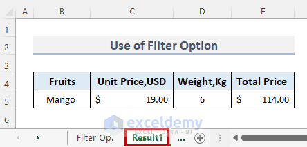
Consider a dataset of some fruits with their unit price, weight, and total price. This full table is saved on a sheet name Filter Op. in our workbook. We will copy the rows from Filter Op. and save them on the Result1 sheet.
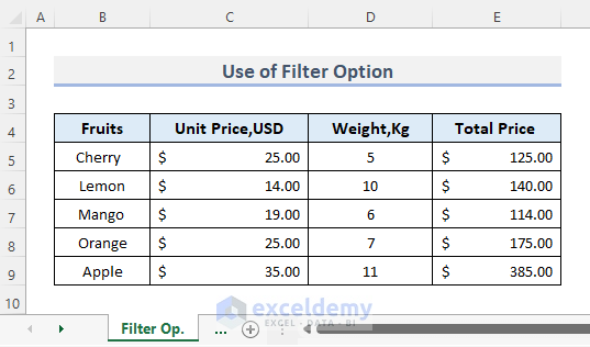
Steps:
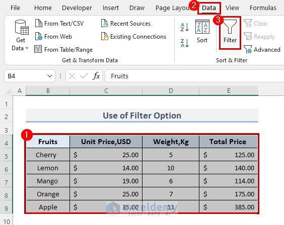
- Select the data.
- Go to the Data tab from the ribbon.
- Click on the Filter option in the Sort & Filter group.
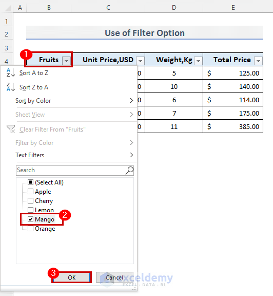
- Select the desired column to which you are going to copy the rows. We have selected the Fruits column.
- Select the row which you want to copy from this Worksheet. We have selected the Mango row for the example. If you need to copy all the rows of this column, choose Select All.
- Select the data and press Ctrl + C.
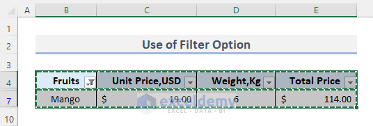
- Create a new worksheet by clicking on the + (plus) sign below or using the keyboard shortcut Shift + F11.
- Paste the copied data by pressing Ctrl + V, into the new worksheet Result1.
- All the selected data will be copied from Filter Op. to Result1.
Method 2 – Utilize the Advanced Filter Feature to Duplicate Rows from One Sheet to Another
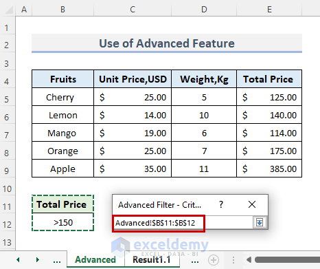
Our testing criteria will be all the fruits whose total price is greater than 150.
Steps:
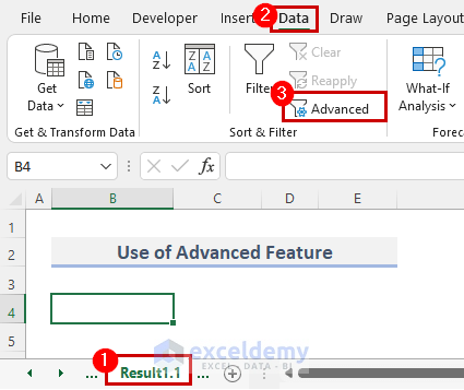
- Go to the Result1.1 sheet and select Advanced under the Data tab.
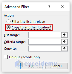
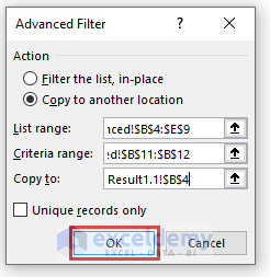
- Select the Copy to another location option.
- Choose the List range box, go to the Advanced sheet, and copy the full dataset.
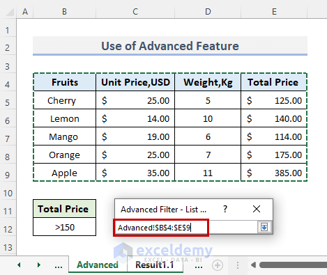
- Pick the Criteria range cell.
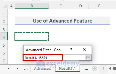
- Select the Copy to option, which will shift automatically to the Result1.1 sheet, and select any cell of that worksheet.
- Press the OK button.
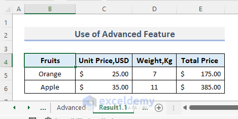
- Rows will be copied from sheet Advanced to Result1.1 based on mentioned criteria.
Method 3 – Copy Rows from One Sheet to Another Using an Array Formula
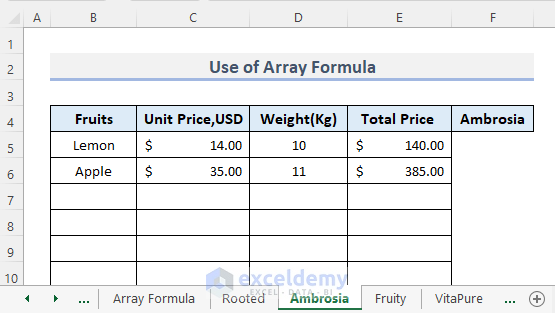
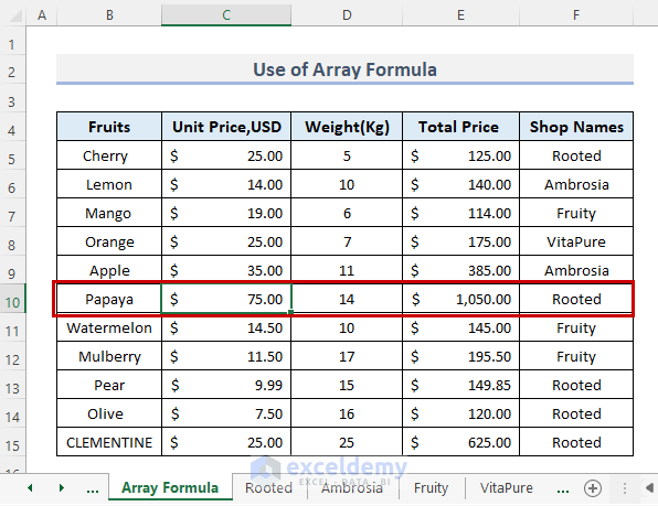
We will copy the rows according to their Shop Names. Each shop will get a separate sheet.
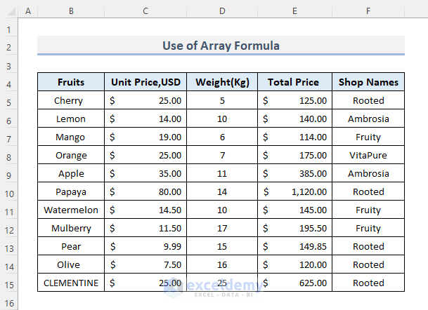
Steps:
- Create new worksheets with the Shop Names.
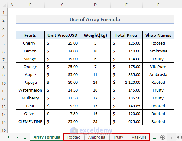
- Go to any new worksheet like Rooted.
- Select cell B5 and enter the following formula, then press Ctrl + Shift + Enter (If you are using MS Excel 365, press Enter).
=IFERROR(INDEX('Array Formula'!$A$5:$E$101,SMALL(IF('Array Formula'!$F$5:$F$101=$C$17,ROW('Array Formula'!$A$5:$B$101)-ROW('Array Formula'!$B$5)+1),ROWS('Array Formula'!$A$5:$B5)),COLUMN()),"")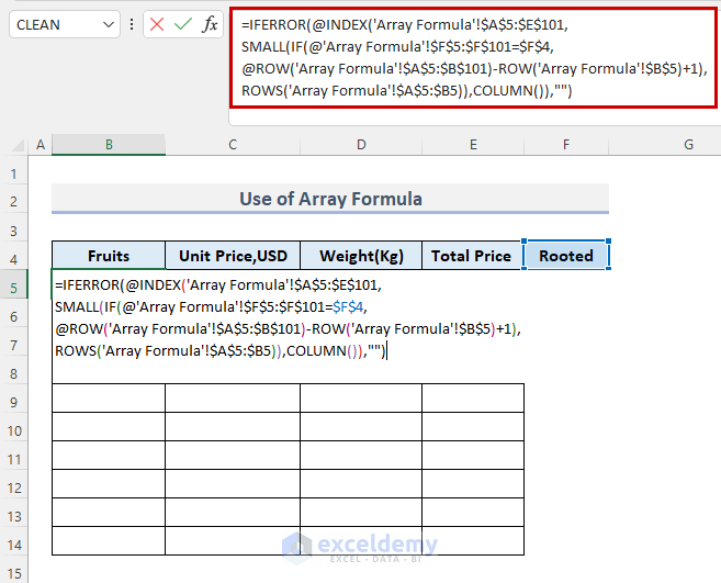
- Copy the formula down and right to get the matched rows.
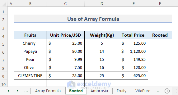
- Do the same for other worksheets.
- Change any value in the Array Formula sheet and the corresponding sheets will be changed. We changed a value in row 10.
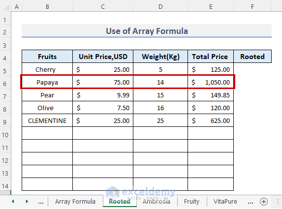
- Go to the Rooted worksheet and see the changes.
Method 4 – Using Combined Functions to Duplicate Rows
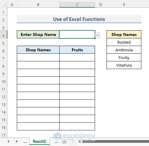
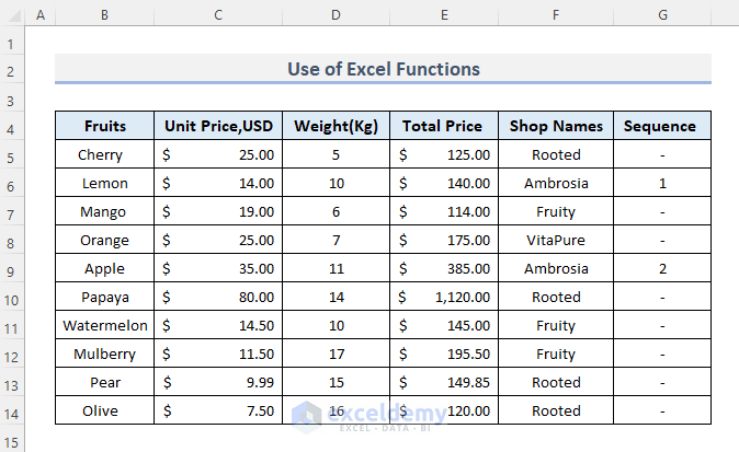
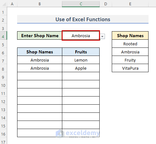
We will sort the list of the fruits according to their Shop Names and check if the Total Price is greater than $130. If we just select any Shop Name from the drop-down list and press Enter, all the matched rows will be copied from the Functions sheet and shown in the Result2 sheet.
STEPS:
- Select the G5 cell in the Functions sheet and enter the following formula:
=IF(AND(F4=Sheet15!$C$1,E4>=130),MAX(G$1:G2)+1,"-")- Press the Enter key from your keyboard.
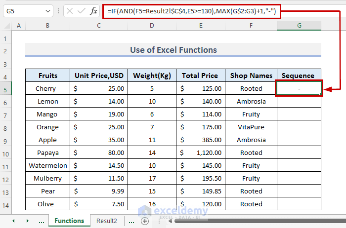
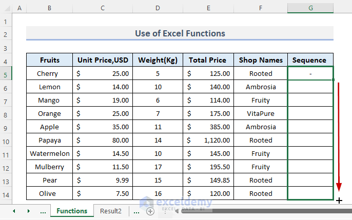
- Drag the Fill Handle icon down to duplicate the formula over the range or double-click on the plus (+) symbol.
- Here’s the result.
- Go to the Result2 sheet and enter the following formula in cell B7.
=IFERROR(INDEX(Sheet14!F:F,MATCH(ROWS($1:1),Sheet14!$G:$G,0))&"","")- Hit the Enter key.
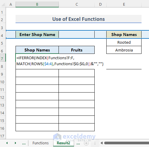
- Copy down and right.
- Select any Shop Name and it will show the Shop Name and Fruit name when the matched Shop Names fruit’s Total Price exceeds $130.
Read More: Copy Rows Automatically in Excel to Another Sheet
Method 5 – Use the FILTER Function to Copy Rows from One Sheet to Another
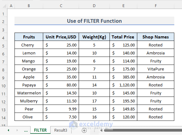
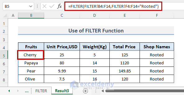
We will take the data from the FILTER sheet that has Rooted under Shop Names and copy it into the Result3 sheet.
STEPS:
- Select the cell where you want to see the result.
- Insert the formula into that cell. In our case, the cell is B5 from sheet Result3.
=FILTER(FILTER!B4:F14,FILTER!F4:F14="Rooted")- Press the Enter key from your keyboard.
Read More: Copy and Paste Thousands of Rows in Excel
Method 6 – Using VBA for Copying Rows from One Sheet to Another
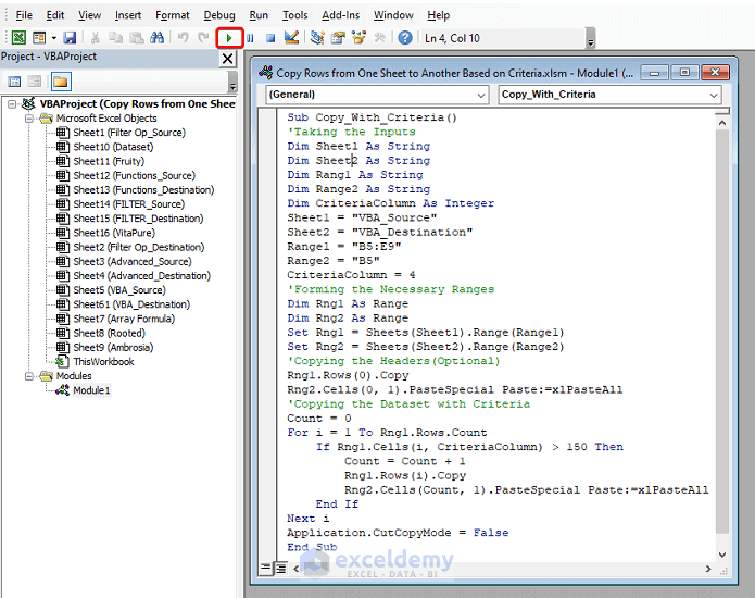
The criteria for copying will be that the total prices have to be greater than $150.
STEPS:
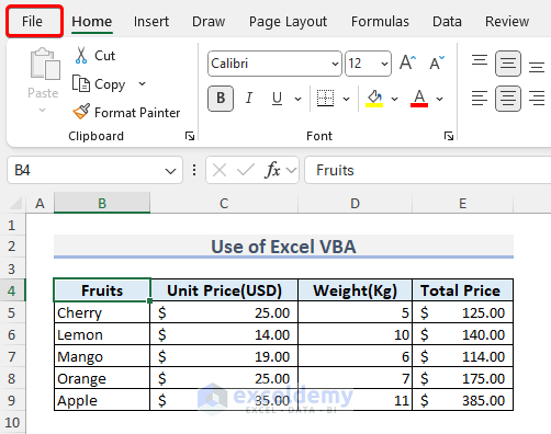
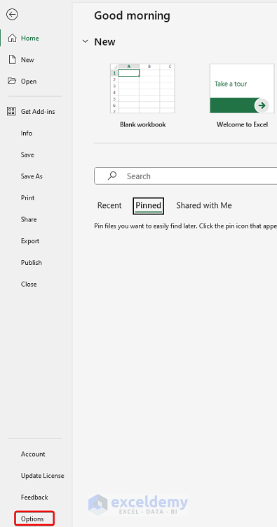
- The Developer tab is not visible by default. To enable it, go to the File.
- Choose Options as shown below.
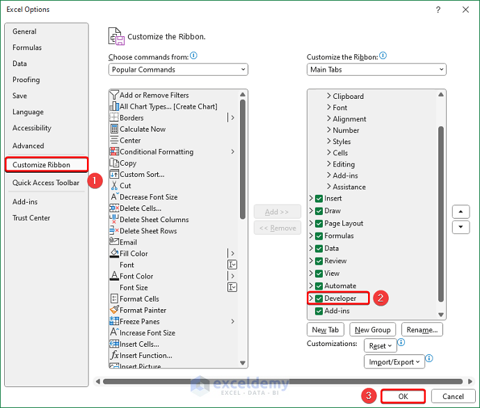
- This will open the Excel Options dialog box. Pick Customize Ribbon.
- Check the Developer box and click OK.
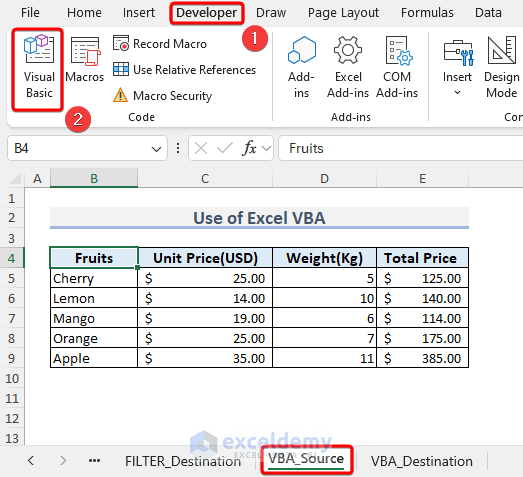
- Go to the Developer tab and click Visual Basic.
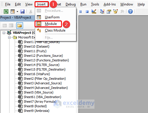
- In the VBA editor, click on Insert and choose Module.
- Insert this VBA code in the Module.
Sub Copy_With_Criteria()
'Taking the Inputs
Dim Sheet1 As String
Dim Sheet2 As String
Dim Rang1 As String
Dim Range2 As String
Dim CriteriaColumn As Integer
Sheet1 = "VBA_Source"
Sheet2 = "VBA_Destination"
Range1 = "B5:E9"
Range2 = "B5"
CriteriaColumn = 4
'Forming the Necessary Ranges
Dim Rng1 As Range
Dim Rng2 As Range
Set Rng1 = Sheets(Sheet1).Range(Range1)
Set Rng2 = Sheets(Sheet2).Range(Range2)
'Copying the Headers(Optional)
Rng1.Rows(0).Copy
Rng2.Cells(0, 1).PasteSpecial Paste:=xlPasteAll
'Copying the Dataset with Criteria
Count = 0
For i = 1 To Rng1.Rows.Count
    If Rng1.Cells(i, CriteriaColumn) > 300 Then
        Count = Count + 1
        Rng1.Rows(i).Copy
        Rng2.Cells(Count, 1).PasteSpecial Paste:=xlPasteAll
    End If
Next i
Application.CutCopyMode = False
End Sub- Click Run.
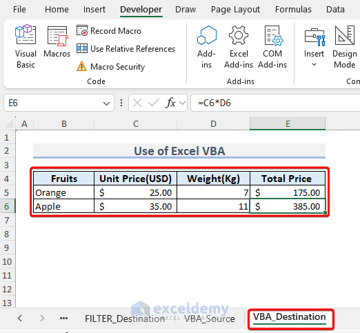
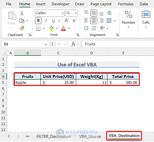
- Go back to the VBA_Destination worksheet.
- You’ll see the rows with the total price greater than $150 have been copied.
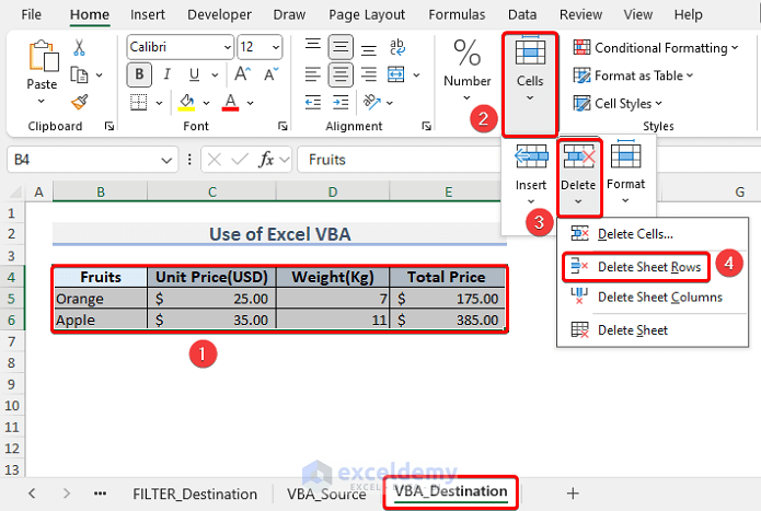
- To change the criteria of total price greater than $150, delete the previously copied rows in the VBA_Destination worksheet.
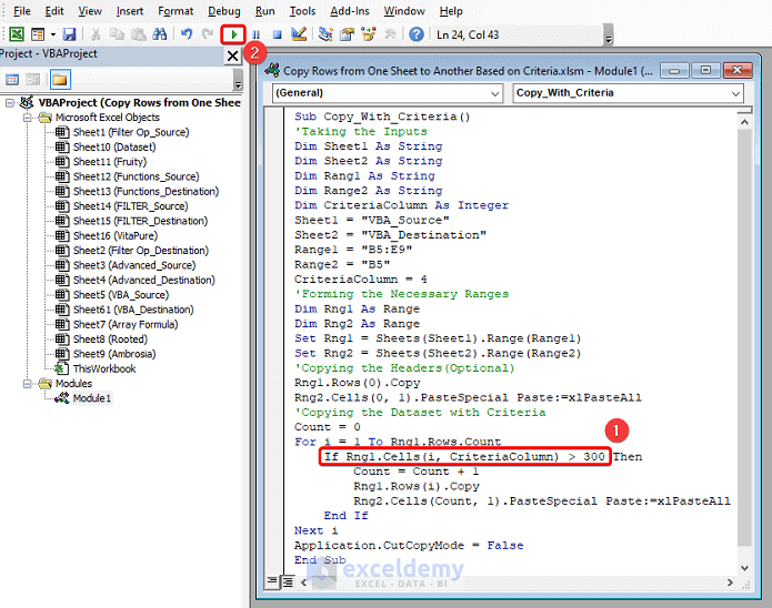
- Edit the criteria as shown in the image below. We’ve changed the criteria to be greater than $300 (>300).
- Press Run.
- Go to the VBA_Destination worksheet to see the results.
Download the Practice Workbook
Related Articles
- Copy Every Nth Row in Excel
- Copy Alternate Rows in Excel
- Copy Rows in Excel with Filter
- Copy Excluding Hidden Rows in Excel
<< Go Back to Copy Rows | Copy Paste in Excel | Learn Excel
Get FREE Advanced Excel Exercises with Solutions!

