Watch Video – TEXT Function to Format Codes in Excel
Method 1 – Joining Texts and Numbers with Excel TEXT Function Format Codes
Below is a dataset of some fruits and their unit price and quantity. The last column is the total price column.
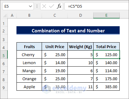
Using the TEXT function, we will calculate the total price using a text and currency symbol, a thousand separator, and two decimal places.
Our formula will be like this:
Formula Explanation:
We add text at the front using the ampersand (&) symbol. Then, in the TEXT function in the first section of the parameters, we will use our formula to count the desired output. After that, put a $ sign at the front for formatting, as the currency symbol here is a dollar, a comma (,) for thousand separators, and a # for representing optional digits.
STEPS:
- Enter the following formula in cell E5:
="Total Price "&TEXT(C5*D5, "$###,###.00")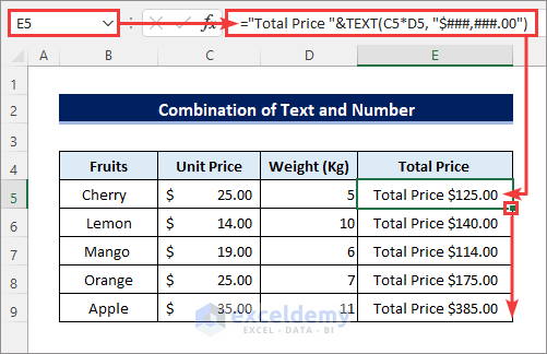
- Drag the Fill Handle icon below to copy the formula.
Read More: How to Combine Text and Numbers in Excel and Keep Formatting
Method 2 – Applying Phone Number Format Codes with TEXT Function in Excel
The below dataset contains some phone numbers for this method. However, the given numbers are not well-formatted.
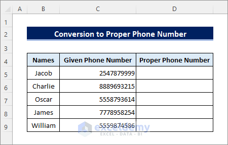
We will convert the mentioned numbers into proper phone numbers using the TEXT function. We want to make phone numbers like this:
(555) 555-1234
- Use a formula as given below:
Formula Explanation:
As we need to format the phone numbers like in the above example, we first need a condition to separate the last 7 digits from the given numbers. We have to use [ ] for conditional purposes. Then we need # for a decimal placeholder to form the number as per our needs.
- In the first section of the TEXT function, it will take the given input, which is our C column. We are taking the given phone numbers without formatting from this column.
- The format section [<=9999999] checks the numbers from the right side to see if it is less than or equal to 7 digits. Then it converts the first 7 digits into ###-#### form which means 3 digit-4 digits pair. After that, the sub-section (###) ###-#### formats the whole number into like this (555) 555-1234. The last 3 digits are covered by (), and the others are 3 digit-4, 4-digit pairs.
- Enter the following formula in cell D5 and then drag the Fill Handle icon below.
=TEXT(C5,"[<=9999999]###-####;(###) ###-####")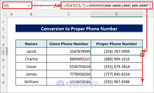
Method 3 – Adding Leading Zeros Before Numbers with Excel TEXT Function
Below is a dataset of some employees with their names and IDs.
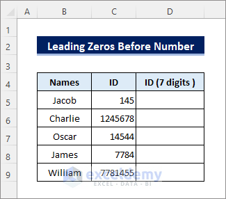
We want to keep all the employees’ IDs in 7 digits, but some are not fully 7 digits. We will convert all the IDs into 7 digits using the format code of the TEXT function.
- Enter the following formula in cell D5 and then drag the Fill Handle icon below.
=TEXT(C5,"0000000")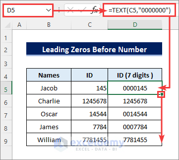
Read More: How to Use Format Function in Excel (with Suitable Examples)
Method 4 – Combining Text and Date Format Codes in Excel with TEXT Function
Below is a dataset of some products and their delivery dates.
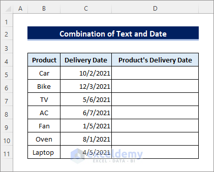
We will combine the products’ names and delivery dates and show them in a single column using TEXT function format codes.
- The syntax of the formula is as follows.
Formula Explanation:
In the above formula, an ampersand (&) operator combines texts. When we need to combine text with text or text with a formula, it’s easily possible in Excel using the ampersand (&). It is the alternative to the CONCAT function in Excel. You can check How to Add Text Before Formula in Excel for more information.
The first section of the parameter takes the values, so as we want to pass the column values of delivery dates, we need to pass the cell number here. In the double quotation, we have declared the formation of dates by using the mm/dd/yyyy format. So, from our given dates, it will format the dates in this format: mm-> month dd-> day yyyy-> year. So, our date will be like this: 05/07/1998.
- Enter the following formula in cell D5 and then drag the Fill Handle icon below.
=B5&"'s delivery date is " &TEXT(C5,"mm/dd/yyyy")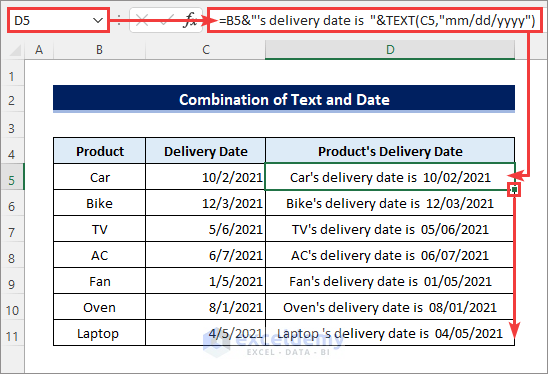
More Examples with Excel TEXT Function to Format Codes
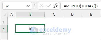
- Let’s calculate today’s month using =MONTH(TODAY()). It will give the current month’s number. Let’s say it’s October, so it will give 10 as the return value.
- But when I use =TEXT(MONTH(TODAY()),”mm”), it returns 01.
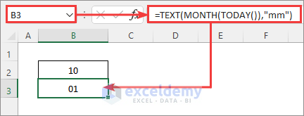
Why Is This Error Happening?
We are converting the date to the number 10, and then you’re telling it to convert the number 10 into a date, which is then known as 02/01/1900 (dd/mm/yyyy), which is the starting numeric value of an Excel date. When you run the text formula, we are getting the 1 from January.
- Another problem is calculating the date and time. If we need to find out both today’s day number and the current hour, we can use the TEXT function. Simply use the formula below.
=TEXT(TODAY(),"dd ") & "Days " & TEXT(NOW(),"hh ") & "Hours"- Using this formula, the first function TEXT(TODAY(),”dd “) calculates today’s date number, and TEXT(NOW(),”hh “) finds out the current hours.

Application of Excel Text Format
Excel can automatically detect the value you try to input into a cell. It will convert the value to the detected format as soon as you enter it, even though you may not want it to do so. Therefore, the intelligence of Excel, which is extremely useful most of the time, may sometimes annoy you.
For example, assume you are trying to enter 5-10 in a cell to indicate 5- 10. However, Excel will treat it as a date. So, it will be entered as Oct 5 or May 10 of the current year, depending on the system date setting. You will face similar annoying results when entering codes with leading zeros. Because Excel will consider the leading zeros as redundancy and remove them automatically.
What do you do to avoid such situations? Well, don’t worry. You can just format the cells as text before entering data. Then, Excel will store values as you input them without any change.
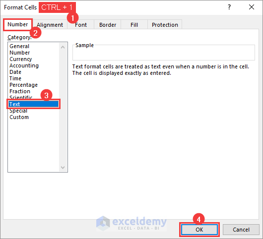
Suppose you want to enter some IDs with leading zeros in B2:B100. Then select the range and press CTRL + 1 or go to Home >> Format >> Format Cells. Next, select the Text category from the Number tab in the Format Cells dialog box and click OK. After that, you can input anything, and Excel will not change anything.
Things to Remember
- Don’t forget to use double quotes around the format codes. Otherwise, the TEXT function will return #NAME! error.
- The TEXT function converts numeric values to text strings. So, you won’t be able to use the output cell as a reference for a numeric value in other formulas. You may need to use other number formats to avoid such limitations if necessary.
Download the Practice Workbook
You can download the workbook to practice.
Related Articles
- How to Use CODE Function in Excel (5 Examples)
- Use CHAR Function in Excel (6 Suitable Examples)
- How to Show Grand Total in Pivot Table (3 Easy Methods)
- Show Percentage in Legend in Excel Pie Chart (with Easy Steps)
- How to Use FIXED Function in Excel (6 Suitable Examples)
- Auto Generate Number Sequence in Excel (9 Examples)
<< Go Back to Excel TEXT Function | Excel Functions | Learn Excel
Get FREE Advanced Excel Exercises with Solutions!

