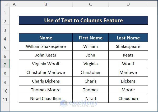
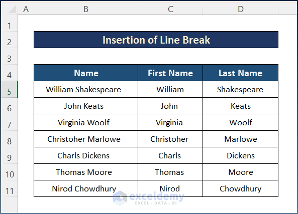
We have a dataset where column B consists of full names. We have to split the cells of column B into two columns, e.g., first name and last name.
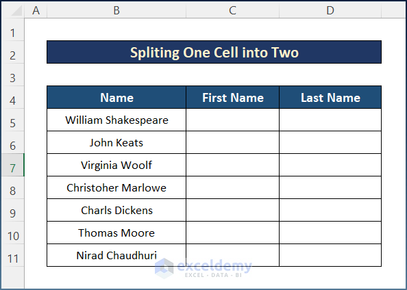
Method 1 – Split One Cell into Two Using the Text to Columns Feature
Steps:
- Select the whole dataset e.g. B4:B11.
- Pick the Text to Columns option from the Data tab.
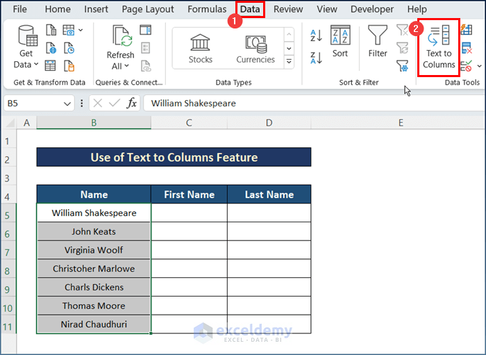
- The Text to Columns Wizard will appear.
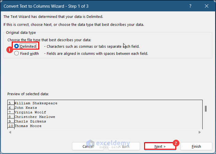
- Choose the Delimited option and press Next.
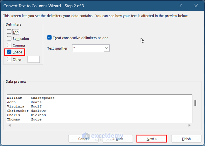
- Select the Space option and press Next.
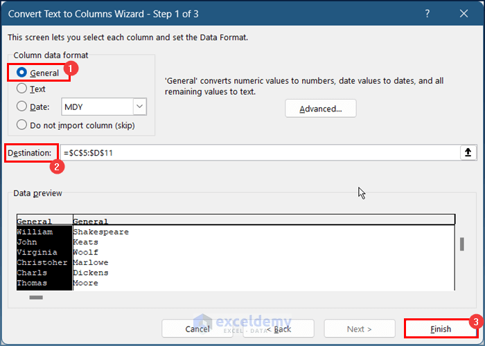
- Select the Text option from the Column Data Format and adjust your Destination if necessary.
- Press Finish.
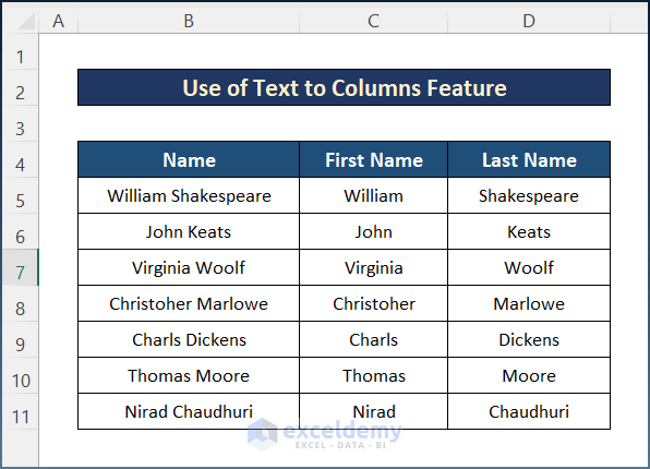
- You will get your final result.
Method 2 – Apply Flash Fill in Excel to Separate Cells
Steps:
- Select a blank cell C5.
- Type in the first name William from the B5 cell in the selected cell C5.
- Use the AutoFill tool for the entire column.
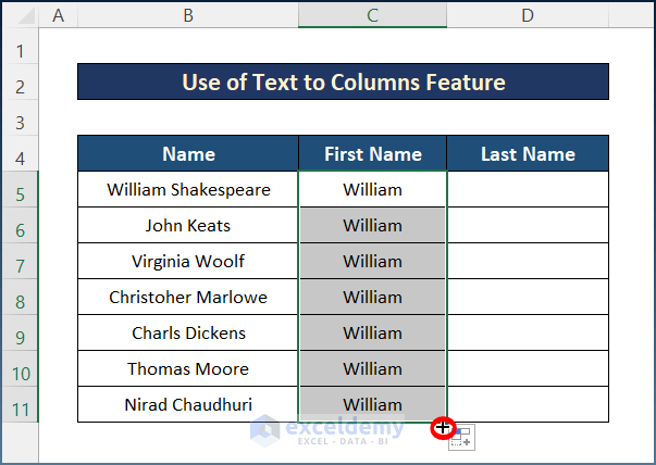
- Select the Flash Fill option to get your desired output.
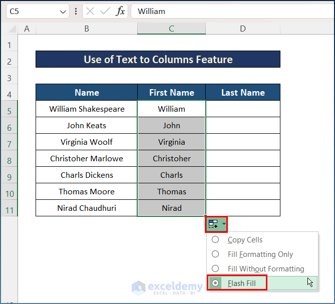
- You can get the same output for the last names by repeating the process for the next column.
Read More: How to Split a Cell into Two Rows in Excel
Method 3 – Insert Formulas for Splitting One Cell into Two in Excel
Case 1 – Use a Delimiter
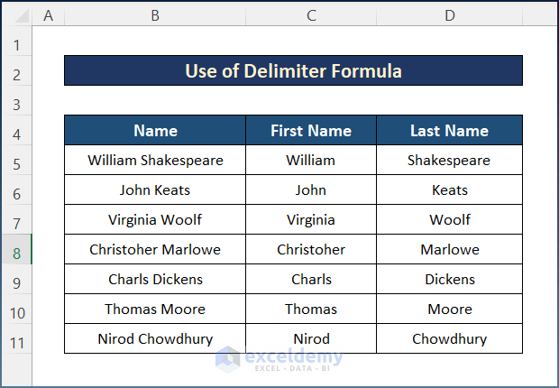
Our dataset uses the space as the delimiter, so we’ll use functions to detect its location and extract the text around it.
Steps:
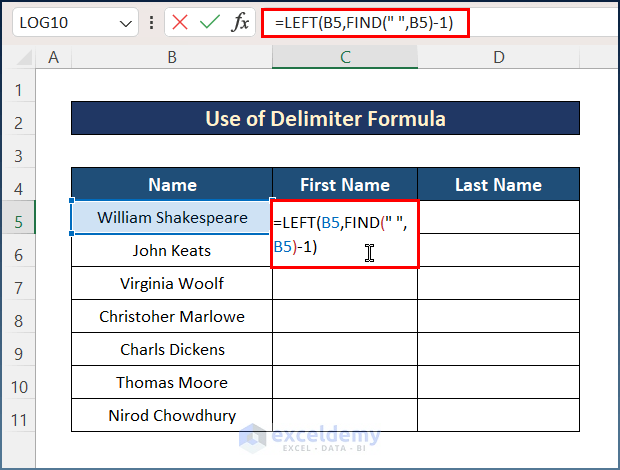
- Select cell C5 and insert the following formula.
=LEFT(B5,FIND(" ",B5)-1)
How Does the Formula Work?
- FIND(” “,B5): The FIND function looks for the space character (“ “) in Cell B5 and returns the position of that character which is ‘8’.
- FIND(” “,B5)-1: After subtracting 1 from the previous result, the new return value here is ‘7’.
- LEFT(B5,FIND(” “,B5)-1): Finally, the LEFT function extracts the 1st 6 characters from the text in Cell B5, which is ‘William’.
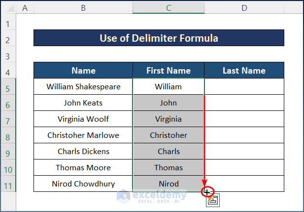
- Press the Enter key and use the AutoFill tool to the entire column.
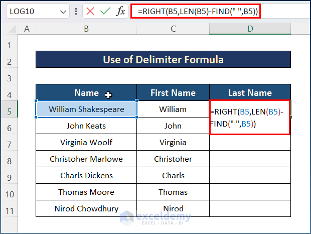
- Use the following formula in cell D5.
=RIGHT(B5,LEN(B5)-FIND(" ",B5))
How Does the Formula Work?
- LEN(B5): The LEN function counts the number of total characters found in cell B5 and thereby returns ‘18’.
- FIND(” “,B5): The FIND function here again looks for the space character in cell B5 and returns the position which is ‘7’.
- LEN(B5)-FIND(” “,B5): This part of the entire formula returns ‘11’ which is the subtraction between the previous two outputs.
- RIGHT(B5,LEN(B5)-FIND(” “,B5)): Finally, the RIGHT function pulls out the last 11 characters from the text in Cell B5 and that is ‘Shakespeare’.
- Use the AutoFill tool to get the final output.
Read More: How to Split a Single Cell in Half in Excel
Case 2 – Insert Line Break
Steps:
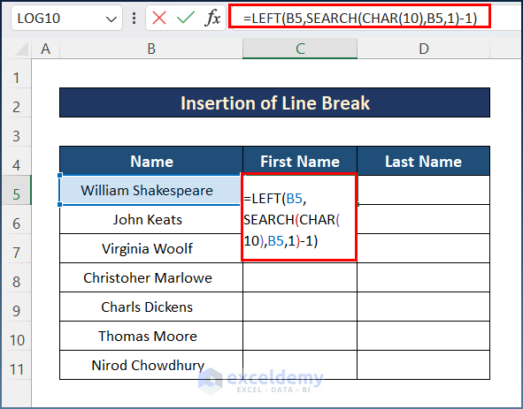
- Insert the following formula in cell C5.
=LEFT(B5,SEARCH(CHAR(10),B5,1)-1)
How Does the Formula Work?
- =SEARCH(CHAR(10),B5,1): This looks for the space character (“ “) in cell B5 and returns ‘9’.
- =LEFT(B5,SEARCH(CHAR(10),B5,1)-1): Finally, the LEFT function extracts the initial characters from the text in cell B5 which is ‘William’.
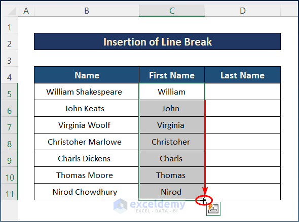
- Hit the Enter key and use the AutoFill tool to the whole column.
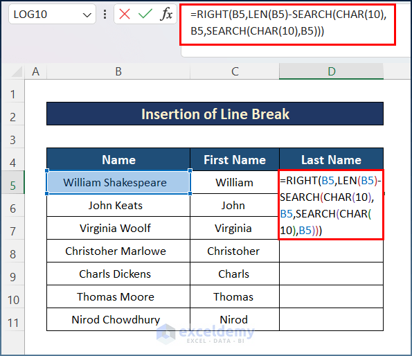
- Insert the formula below in cell D5.
=RIGHT(B5,LEN(B5)-SEARCH(CHAR(10),B5,SEARCH(CHAR(10),B5)))
How Does the Formula Work?
- =SEARCH(CHAR(10),B5): This looks for the space character (“ “) in Cell B5 and returns ‘9’.
- SEARCH(CHAR(10),B5,SEARCH(CHAR(10),B5)): also returns ‘9’.
- =RIGHT(B5,LEN(B5)-SEARCH(CHAR(10),B5,SEARCH(CHAR(10),B5))the ): Finally, the RIGHT function extracts the last characters from the text in cell B5 which is ‘Shakespeare’.
- Press the Enter key and use the AutoFill tool to get the final output.
Read More: Excel Formula to Split String by Comma
Method 4 – Combine RIGHT, SUM, LEN, and SUBSTITUTE Functions to Split Cells
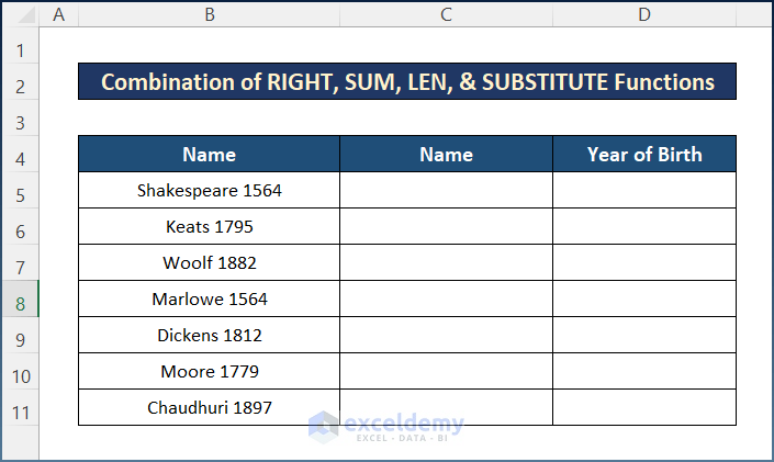
We changed the dataset slightly to include a mix of names and numbers (the year of birth) in the order “Name DoB.”
Steps:
- Select cell D5 and insert the following formula.
=RIGHT(B5,SUM(LEN(B5) - LEN(SUBSTITUTE(B5,{"0","1","2","3","4","5","6","7","8","9"},""))))
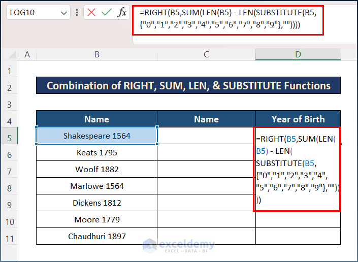
- Press Enter and apply the AutoFill tool.
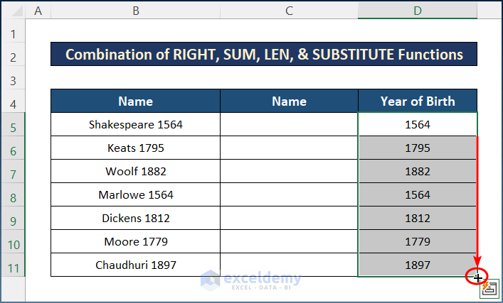
- Use the following formula in cell C5.
=LEFT(B5,LEN(B5)-LEN(D5))
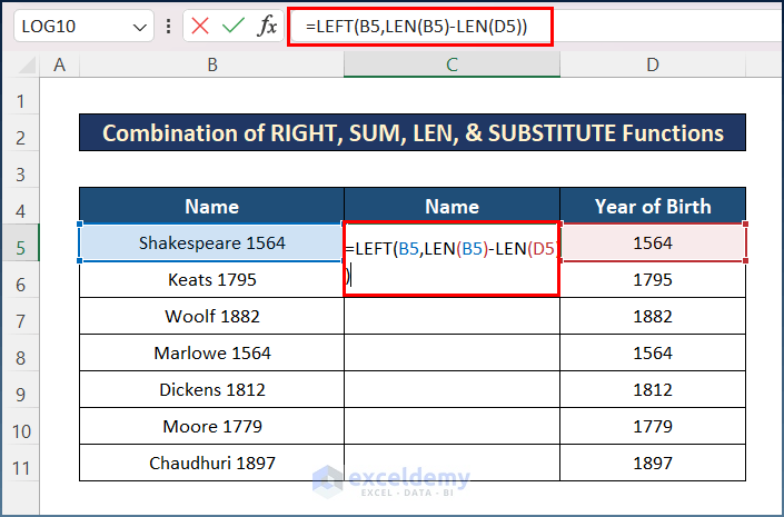
- Hit the Enter key and apply the AutoFill tool to get the desired output.
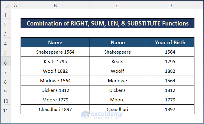
Method 5 – Break One Cell into Two Through Excel Power Query
Steps:
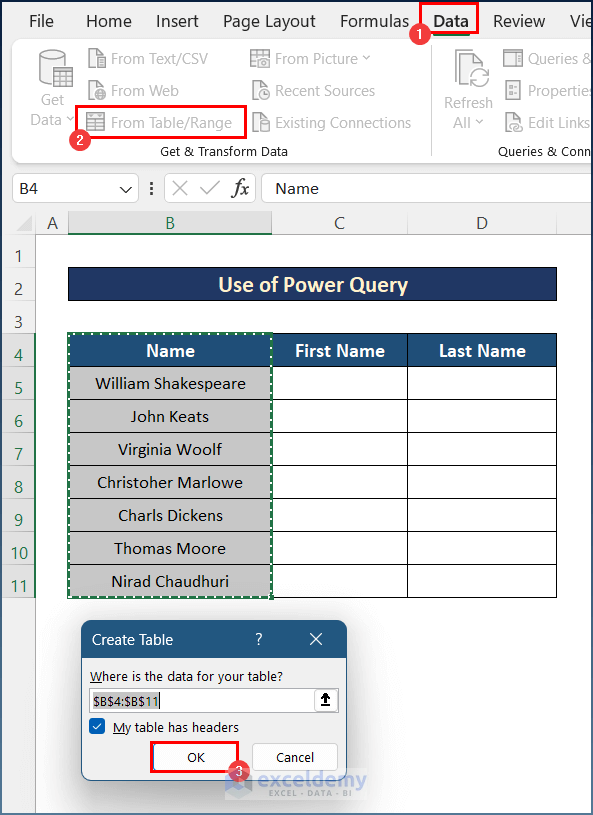
- Select the entire column, including the header.
- Go to the Data tab and click on From Table/Range.
- Press OK.
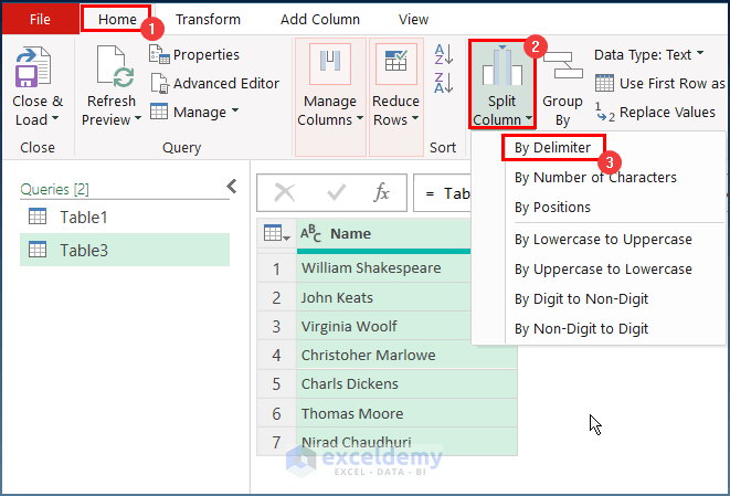
- You’ll get the Power Query Editor,
- Go to Home, select Split Column, and choose By Delimiter.
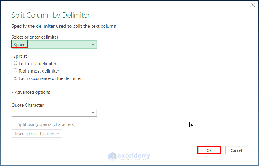
- Select Space as your delimiter and press OK.
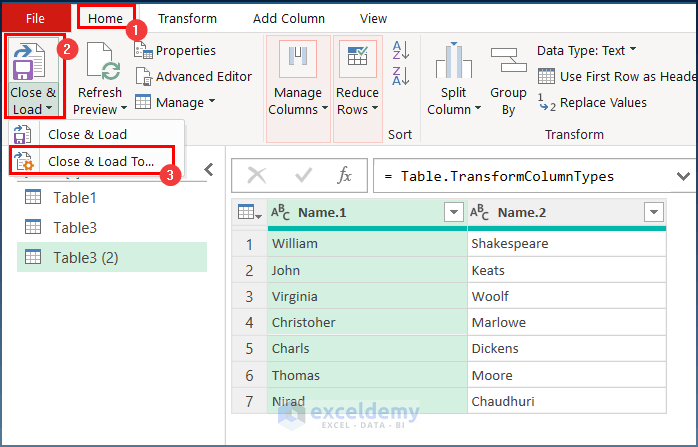
- Click on Close & Load, then on Close & Load To.
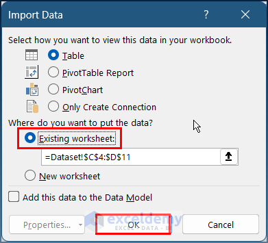
- Choose your destination in the Import Data dialog box and press OK.
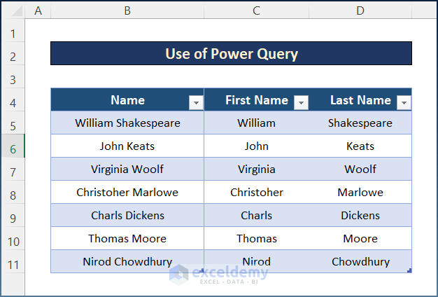
- Here’s the output.
Read More: How to Split Cell by Delimiter Using Excel Formula
Download the Practice Workbook
Get FREE Advanced Excel Exercises with Solutions!

