How to Fix If SUMIFS Is Not Working with Multiple Criteria (3 Solutions)

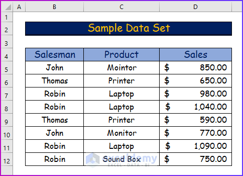
Below is a sample dataset of random information regarding the sales of some products.

Solution 1 – Giving Proper Criteria Range

Steps:

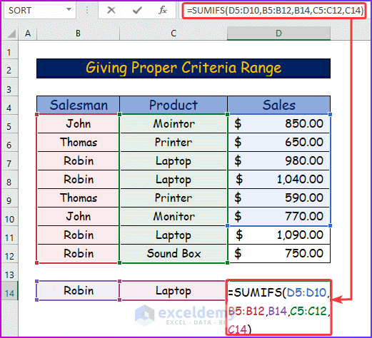
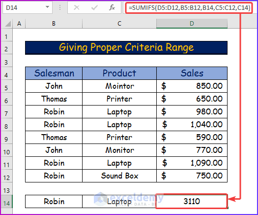
• In cell D14, insert the following SUMIFS function formula:

• The formula shows that the proper sum range is missing.
• The actual sum range is D5:D12, while in the formula it is D5:D10.

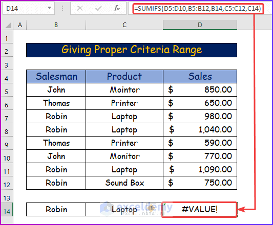
• Press Enter, and you will get #VALUE! as a result.

To solve the error,

• Enter the following formula by mentioning the proper sum range which is D5:D12:

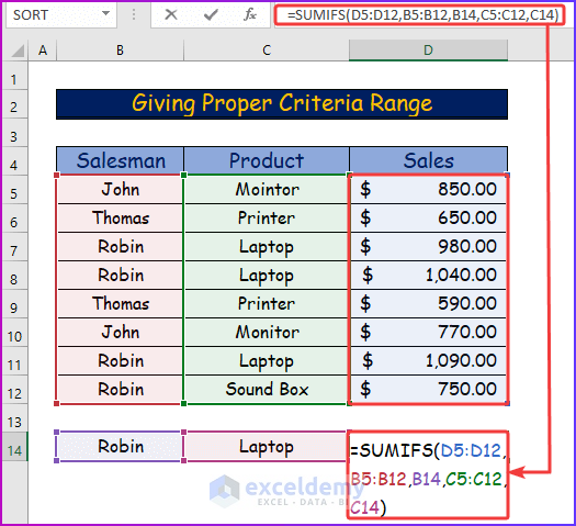
• Press Enter to get the result.

Read More: Excel SUMIFS Not Equal to Multiple Criteria

Solution 2 – Inserting a Proper Sign

Steps:

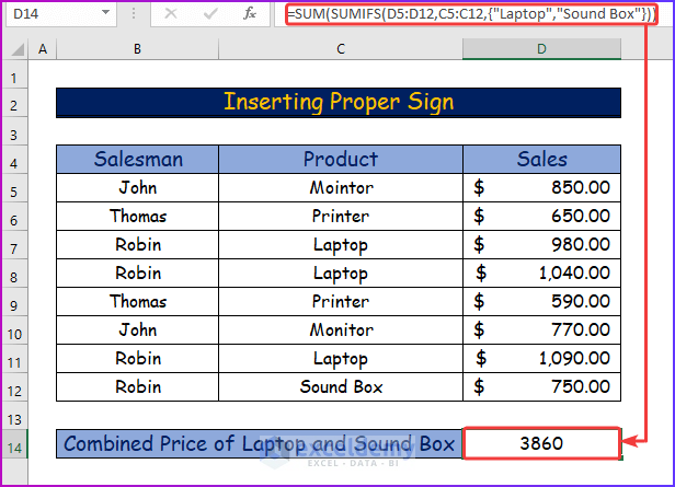
• In cell D14, we will use the data set to determine the combined price of the laptop and sound box.
• Enter the following formula in cell D14:

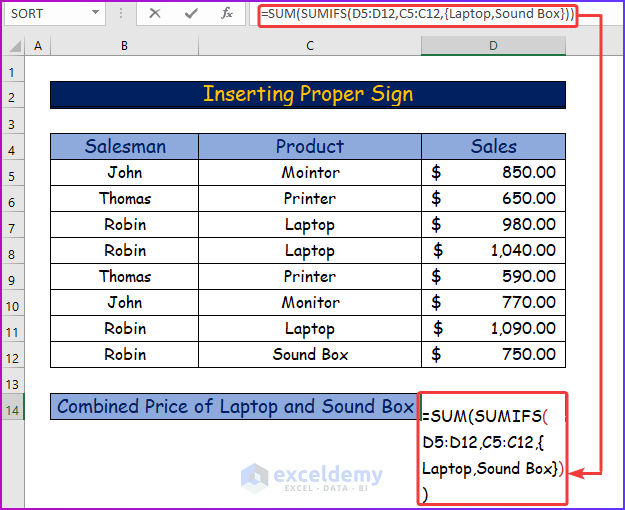
In the above formula, I did not use a double quotation mark inside the second bracket.

• Input the required symbol because both criteria are in text formats.
• When you press Enter after typing the above formula, you will get an error message like the following image.

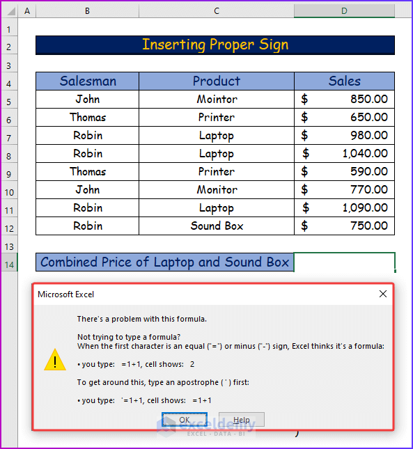
To solve the issue,

• Enter the formula in the following format by adding a double quotation inside the second bracket:

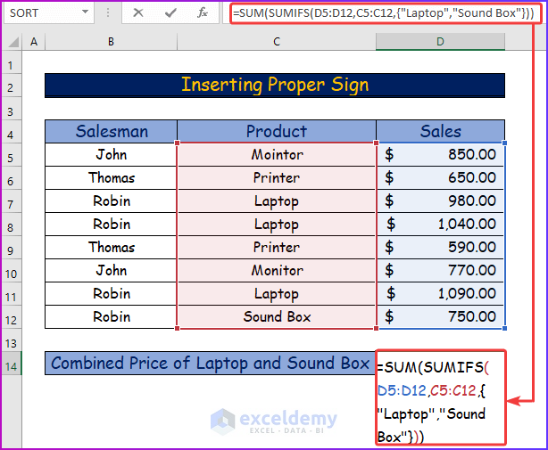
• Press Enter to get the desired result.

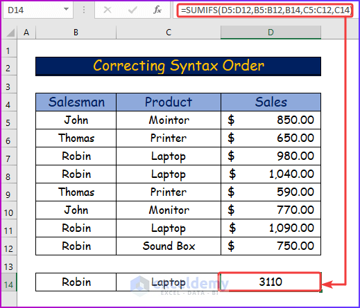
Solution 3 – Correcting Syntax Order

Steps:

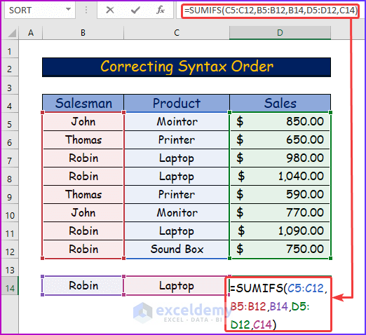
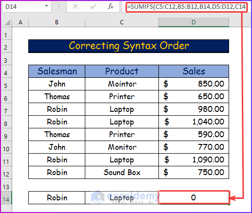
• Look at the formula of the SUMIFS function in cell D14.

• In the function syntax, cell range C5:C12 is one of the criteria ranges, not a sum range.
• The actual sum range of this function is D5:D12, which is mentioned at the end of the syntax.

• Press Enter with this error will result in a 0 like the following image.

• Correct the syntax of this formula by placing the sum range at the beginning.

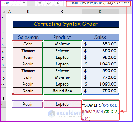
• Press Enter to get the result.

Applying the SUMIFS Function with Multiple Criteria in the Same Column

Steps:

• Take the following data set for calculation.
• I want to know the sales of laptops and sound boxes from column C, which is associated with the salesman Robin from column B.
• From column C, I am selecting more than one criterion.

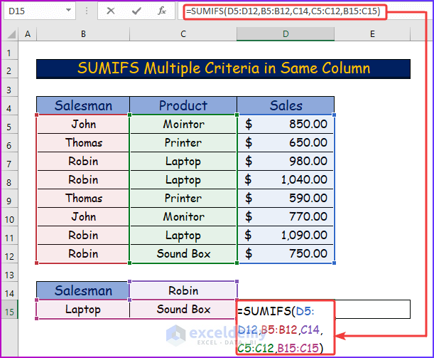
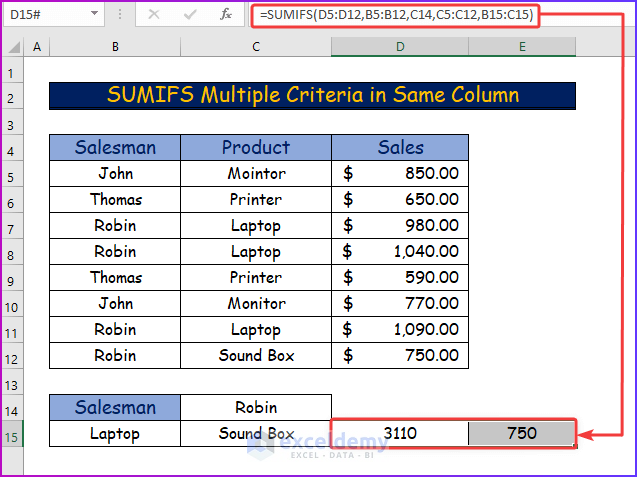
• Enter the following formula in cell D15:

• Here, I referred to multiple criteria from both column and row.

• Press Enter, and the formula will show the result of sales for both the laptop and the sound box separately.

Read More: Excel SUMIFS with Multiple Sum Ranges and Multiple Criteria

Download the Practice Workbook

You can download the free Excel workbook here and practice on your own.

Related Articles

• How to Use SUMIFS Function with Multiple Sheets in Excel
• SUMIFS with INDEX-MATCH Formula Including Multiple Criteria
• How to Use SUMIFS Function with Wildcard in Excel

<< Go Back to Excel SUMIFS with Multiple Criteria | Excel SUMIFS Function | Excel Functions | Learn Excel