[Solved] SUMPRODUCT with Multiple Criteria Not Working in Excel (3 Solutions)

Example 1 – If the Specified Arrays Are Not Same

One of the biggest problems users face while dealing with the SUMPRODUCT function is when they fail to input the same dimension of arrays. In the following sample dataset, we have column headers for Branch Number, Quantity and Price Per Unit. We need to find the total price of all quantities in cell D17.

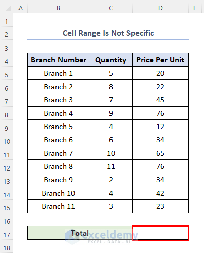
Enter the following SUMPRODUCT function in the D17 cell.

=SUMPRODUCT(C5:C15,D5:D12)

C5:C15 refers to the Quantity of Fruit Items and D5:D12 refers to the Price Per Unit of the Quantities from D5 cell to D12 cell.

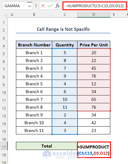
Press ENTER.

The output will be #VALUE!.

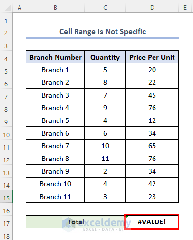
The ranges used in the SUMPRODUCT function should be equal in Rows. We have used C5:C15 as the first range, which has 11 Rows, and D5:D12 as the second range with 8 Rows. These two ranges don’t have an equal number of Rows. This is the reason why the SUMPRODUCT function has given an error as output.

Solution:

We have to take an equal number of Rows as ranges.

Enter the following formula in the D17 cell.

=SUMPRODUCT(C5:C15,D5:D15)

The number of Rows of the two ranges are equal, i.e. 11 rows.

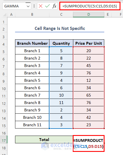
Press ENTER.

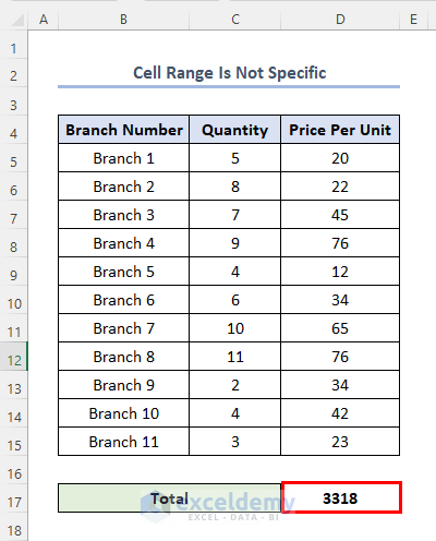
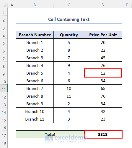
The output becomes valid and result is 3318.

Example 2 – If Any Cell Contains Text

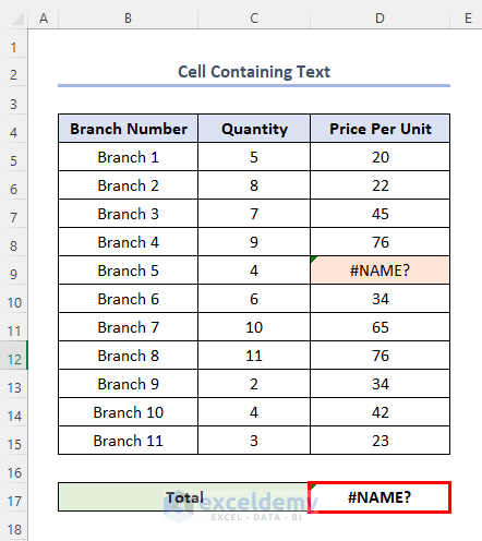
When one or more cells in the referenced range contain text or are formatted as a text data type, we’ll get a #VALUE! Error or #NAME? Error. The text could be the result of a calculation from another formula. Another reason could be that the cell is not formatted correctly.

Suppose we have a text in the D9 cell, and other cells in the same Column contain General Numbers. We need to find the total price of all quantities in cell D17.

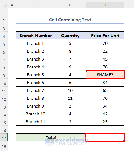
Enter the following formula in the D17 cell.

=SUMPRODUCT(C5:C15,D5:D15)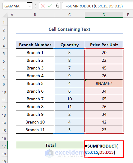

On pressing ENTER, we’ll see the output as #Name!.

Solution:

If we replace the text of the D9 cell with a General Number, we’ll get a valid output. We have replaced the text with 12 and we will get the output 3318.

Related Content: Excel SUMPRODUCT Function Based on Date Range

Example 3 – If Formula Has Error in 3D Reference

If we use the SUMPRODUCT function and take ranges from single or multiple sheets and these sheet names are included in Name Manager as names, we’ll face errors while using it.

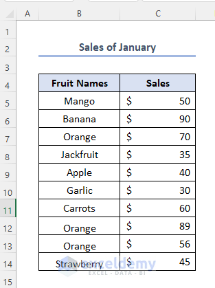
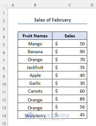
Suppose we have 3 datasets of Sales of Fruits in individual months.

The first dataset is the Sales of January.

The second dataset is the Sales in February.

The third dataset is the Sales in March.

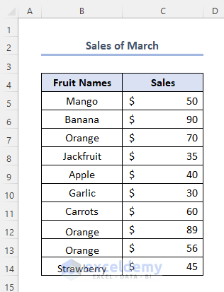
We will find the Total Sales of individual fruits throughout the three months.

For Mango, enter the following formula using the SUMPRODUCT function.

=SUM(SUMPRODUCT('Jan'!B5:B14='Using SUMPRODUCT'!B5)*' Jan'!C5:C14),

SUMPRODUCT((' Feb'!B5:B14='Using SUMPRODUCT'!B5)*Feb!C5:C14),

SUMPRODUCT((Mar!B5:B14='Using SUMPRODUCT'!B5)*Mar!C5:C14))

Jan’!B5:B14 is the range of Fruit Names in the Jan sheet, Feb’!B5:B14 is the range of Fruit Names in the Feb sheet and Mar!B5:B14 is the range of Fruit Names in the Mar sheet.

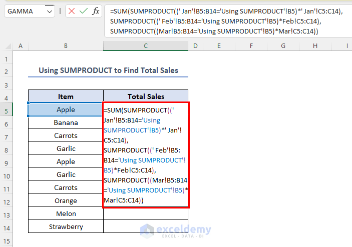Press ENTER and use the Fill Handle for the rest of the cells.

The output will be #REF!

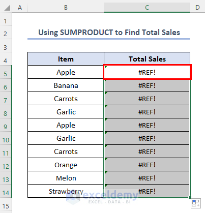
This error is occurring because we have added Jan, Feb and Mar as references by using the Name Manager in the Formula bar.

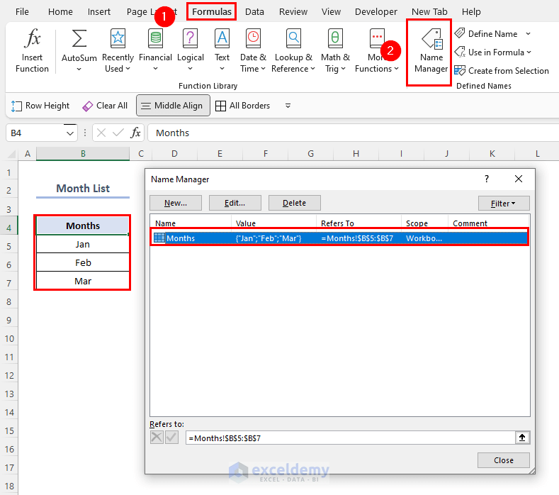
The names of our reference sheets are Jan, Feb, and Mar as well.

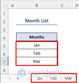
What happens here is that the SUMPRODUCT function cannot understand the reference because we have added a Name Manager, which is the same as Sheet Names. So, Excel takes Jan, Feb and Mar as references from the Name Manager. This is the reason why we get the output #REF!

Solution:

To avoid this error, we must not use the same names as Sheet Names and as references in the Name Manager.

When we don’t include the same name reference as the sheet name through Name Manager, we’ll find the valid output as 210 for Mango and other outputs after using the Fill Handle.

Read More: How to Use SUMPRODUCT IF in Excel

Things to Remember

Non-numeric array entries will be treated as zeroes by the SUMPRODUCT function.
In Excel 2016, Excel 2013, Excel 2010, and Excel 2007, SUMPRODUCT supports up to 255 arguments, while prior Excel versions only supported 30 arguments.
Arrays will provide TRUE and FALSE values as a result of logical testing. Most of the time, it is best to convert them to 1s and 0s.
The SUMPRODUCT formula treats all the non-numeric values as zero.
The SUMPRODUCT formula will return an error if it is not double-negative signed or multiplied by one.