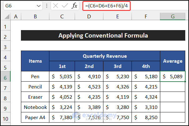
Consider the dataset of the quarterly revenue report of a stationary company for 5 different items.

Method 1 – Applying a Conventional Formula
Steps:
- Select G6.
- Enter the following formula in the cell.
=(C6+D6+E6+F6)/4
- Press Enter.
- Drag down the Fill Handle to see the result in the rest of the cells.
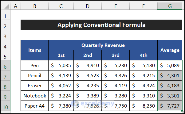
You will see the average value of the quarterly revenue.

Read More: How to Calculate Monthly Average from Daily Data in Excel
Method 2 – Using the AVERAGE Function
Steps:
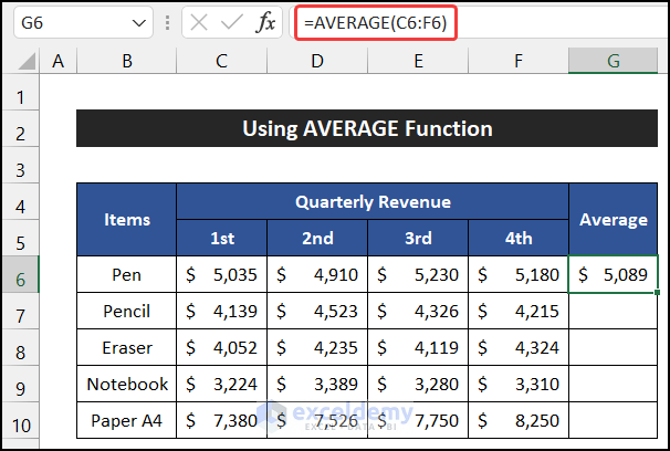
- Select G6.
- Enter the following formula in the cell.
=AVERAGE(C6:F6)
- Press Enter.
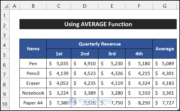
- Drag down the Fill Handle to see the result in the rest of the cells.

You will see the average value of the quarterly revenue.
Read More: How to Calculate Average Revenue in Excel
Method 3 – Utilizing the AVERAGEA Function
Steps:
- Select G6.
- Enter the following formula in the cell.
=AVERAGEA(C6:F6)
- Press Enter.

- Drag down the Fill Handle to see the result in the rest of the cells.
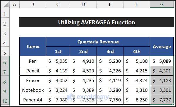
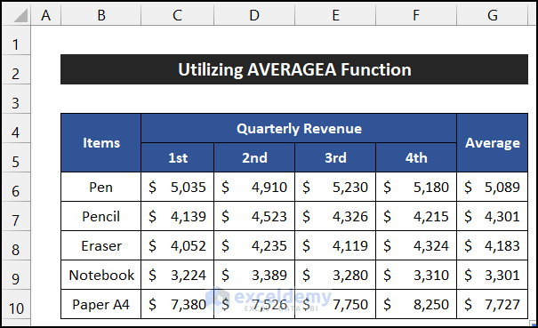
You will see the average value of the quarterly revenue.
Read More: Moving Average Formula in Excel
Method 4 – Combining the AVERAGE and the LARGE Functions
Steps:
- Select G6.
- Enter the following formula in the cell.
=AVERAGE(LARGE(C6:F6,{1,2,3,4}))
- Press Enter.

- Drag down the Fill Handle to see the result in the rest of the cells.
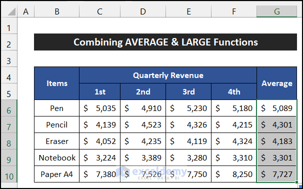
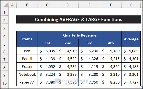
You will see the average value of the quarterly revenue.
Formula Breakdown
LARGE(C7:F7,{1,2,3,4}): returns 4523, 4326, 4215, and 4139.
AVERAGE(LARGE(C6:F6,{1,2,3,4})): returns the average of the four numbers of the array and shows the final result: 5089.
Method 5 – Combining the AVERAGE and the SMALL Functions
Steps:
- Select G6.
- Enter the following formula in the cell.
=AVERAGE(SMALL(C6:F6,{1,2,3,4}))
- Press Enter.
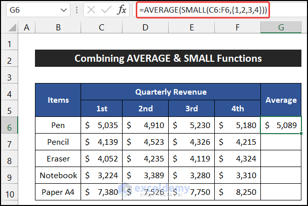
- Drag down the Fill Handle to see the result in the rest of the cells.

You will see the average value of the quarterly revenue.
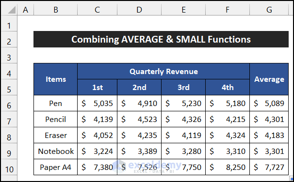
Formula Breakdown
SMALL(C6:F6,{1,2,3,4}): returns 4910, 5035, 5180, and 5230.
AVERAGE(SMALL(C6:F6,{1,2,3,4})): returns the average of the four numbers of the array and shows the final result: 5089.
Method 6 – Using the AutoSum to Find the Average
Steps:
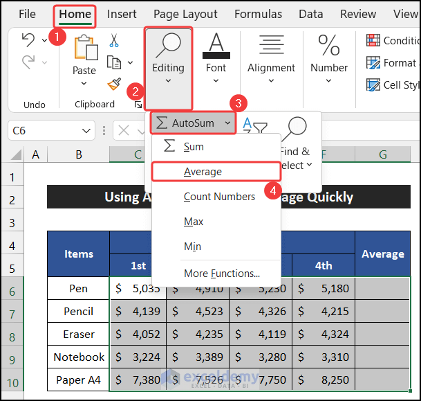
- Select C6:G10.
- In the Home tab, select AutoSum > Average in Editing.
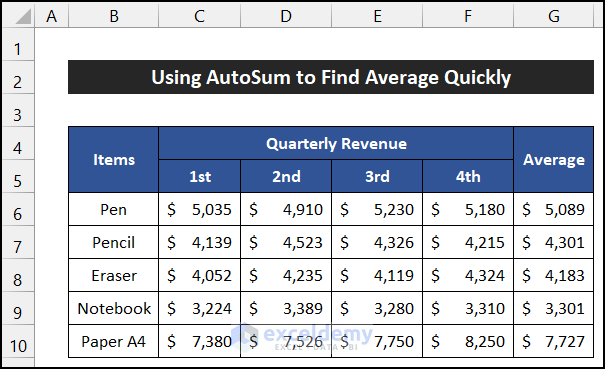
You will see the average value of the quarterly revenue.
Read More: How to Calculate Average of Multiple Ranges in Excel
Method 7 – Estimating the Average with the SUM Function
Steps:
- Select G6.
- Enter the following formula in the cell.
=SUM(C6:F6)/4
- Press Enter.
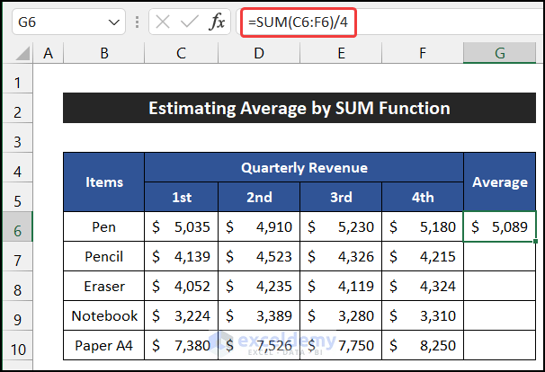
- Drag down the Fill Handle to see the result in the rest of the cells.

You will see the average value of the quarterly revenue.

Read More: How to Calculate Sum & Average with Excel Formula
Method 8 – Calculating the Average with the SUBTOTAL Function
Steps:
- Select G6.
- Enter the following formula in the cell.
=SUBTOTAL(9,C6:F6)/4
- Press Enter.
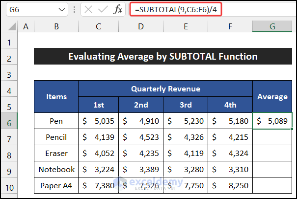
- Drag down the Fill Handle to see the result in the rest of the cells.
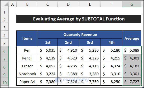
You will see the average value of the quarterly revenue.

Read More: How to Do Subtotal Average in Excel
Download Practice Workbook
Download the practice workbook.
Related Articles
- Average Attendance Formula in Excel
- How to Calculate Average, Minimum And Maximum in Excel
- How to Calculate Average of Averages in Excel
- How to Calculate Average True Range in Excel
- How to Calculate Average Percentage in Excel
- How to Calculate Average Percentage of Marks in Excel
- How to Calculate Class Average in Excel
- How to Calculate Average Share Price in Excel
- How to Calculate Average Length of Stay in Excel
- How to Calculate Average Price in Excel
<< Go Back to Excel Average Formula Examples | How to Calculate Average in Excel | How to Calculate in Excel | Learn Excel
Get FREE Advanced Excel Exercises with Solutions!

