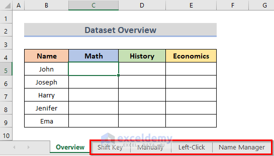
Dataset Overview
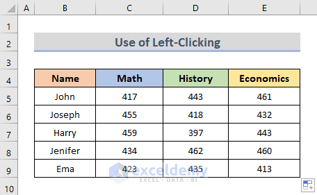
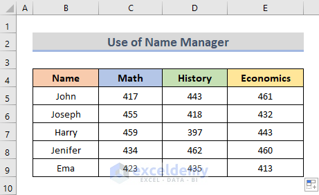
To demonstrate these methods, we’ll use a dataset (B4:E9) containing student names and marks for Math, History, and Economics.
Method 1 – Calculate Data Across Worksheets Using Excel Formula with Shift Key
We will use the SUM function to calculate the total marks in Math for all the tests.
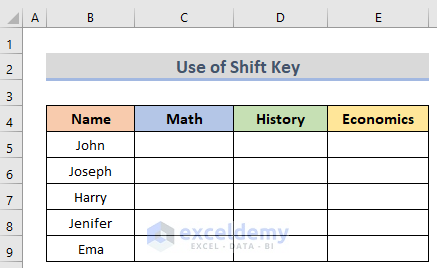
Steps
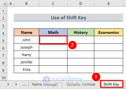
- Click the Shift Key tab at the bottom of the worksheet.
- Select cell C5.
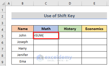
- Enter the SUM function in cell C5.
- Click on the Test1 sheet tab.
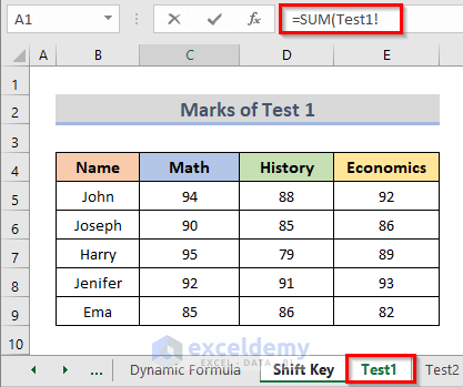
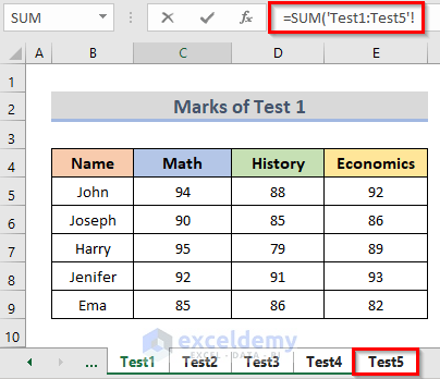
- Hold down the Shift key and click on the Test5 tab.
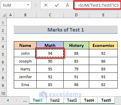
- Select cell C5 of the Test1 worksheet.
- Close the parentheses in the Formula Bar.
- The final formula is:
=SUM(‘Test1:Test5’!C5)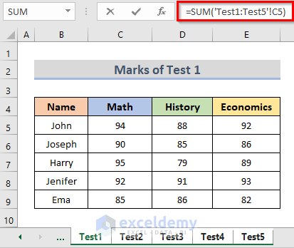
- Press Enter to get the result in cell C5.
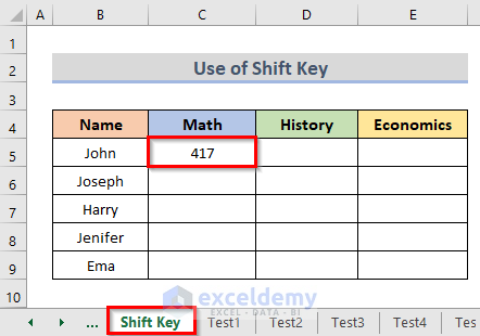
- Drag the fill handle to the right (up to cell E5) to copy the formula for all subjects.
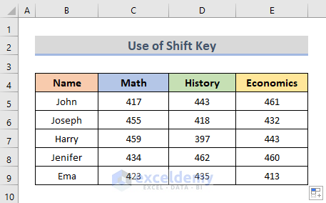
- Select C5:E5 and double-click on the plus sign to autofill the next cells.
- We have calculated the total marks for all subjects (see the picture below).
Method 2 – Manually Insert Formulas to Calculate Data for Several Excel Worksheets
Steps
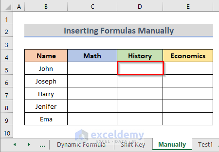
- Go to cell D5.
- To calculate the total marks for History, enter this formula in cell D5:
=Test1!D5+Test2!D5+Test3!D5+Test4!D5+Test5!D5- Press Enter.
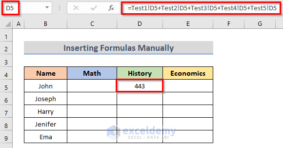
- Drag the fill handle up to cell D9.
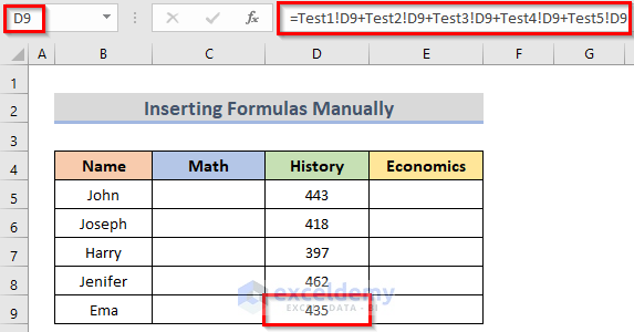
- Calculate the total marks for Math (cell C5):
=Test1!C5+Test2!C5+Test3!C5+Test4!C5+Test5!C5- Calculate the total marks for Economics (cell E5):
=Test1!E5+Test2!E5+Test3!E5+Test4!E5+Test5!E5- The final result is in the picture below.
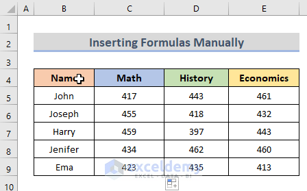
Method 3 – Apply Formula Across Excel Worksheets with Left-Click to Get Data
Steps
- Go to the Left-Click sheet tab.
- Enter the SUM function in cell E5.
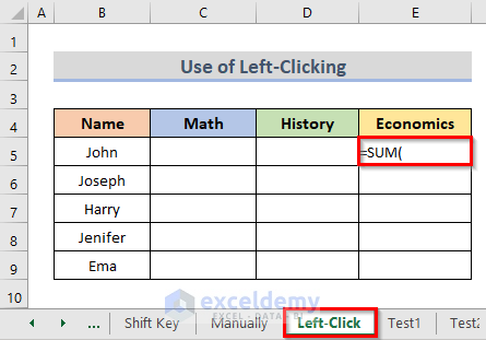
- Click on the Test1 sheet tab and confirm it’s inserted in the formula.
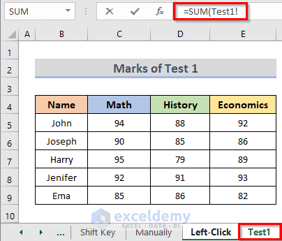
- Click on cell E5 of the Test1 worksheet.
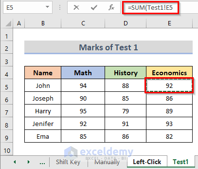
- Add a comma (,) to the formula (see the Formula Bar of the screenshot below).
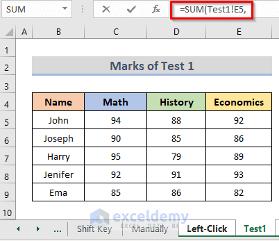
- Complete the formula for other worksheets.
- The entire formula is:
=SUM(Test1!E5,Test2!E5,Test3!E5,Test4!E5,Test5!E5)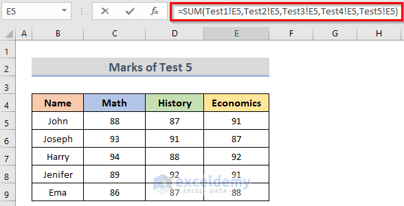
- Press Enter to calculate John’s total marks in Economics (cell E5).
- Double-click the fill handle to calculate Economics marks in the range E6:E9.
- Repeat the process for Math (cell C5) and Economics (cell E5).
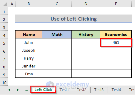
- Double-click on the fill handle to calculate the total marks for Economics in the range E6:E9.
- Generate the formula below in cell C5 to find the total marks for Math:
=SUM(Test1!C5,Test2!C5,Test3!C5,Test4!C5,Test5!C5)- For Economics, enter the formula below in cell E5:
=SUM(Test1!E5,Test2!E5,Test3!E5,Test4!E5,Test5!E5)- We can see the final output in the following screenshot.
Method 4 – Use the Name Manager Feature to Generate Formulas for Multiple Sheets in Excel
Steps
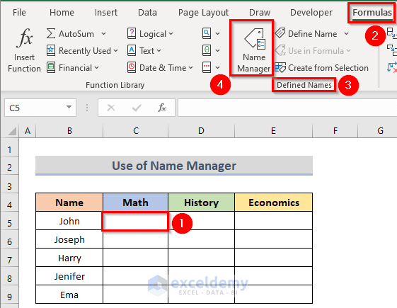
- Select cell C5.
- Go to the Formulas tab.
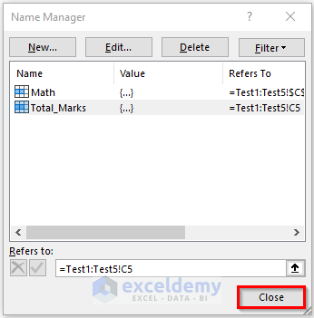
- Within Defined Names group > click on Name Manager.
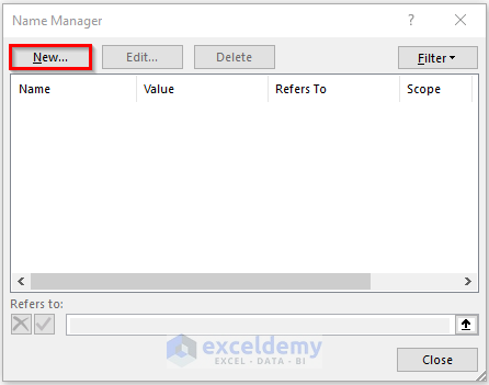
- In the Name Manager window, click on the New button.
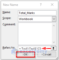
- In the New Name window:
- Enter a name (e.g., Total_Marks) without spaces.
- In the Refers to field, enter the following formula:
=’Test1:Test5’!$C$5This formula refers to cell C5 across the worksheets named Test1 through Test5.
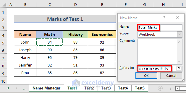
- Remove the dollar sign ($) from the formula to make it relative. This allows you to use it for other cells.
- Click OK to create the new name.
- Close the Name Manager window.
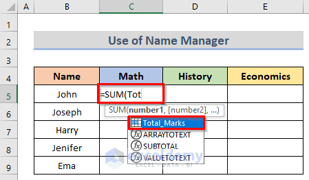
- Go back to cell C5. Enter the SUM function, and you’ll see the Total_Marks option appear below cell C5.
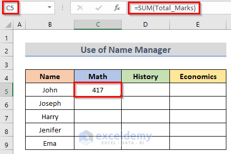
- The formula will look like this:
=SUM(Total_Marks)- Press Enter to calculate the result in cell C5.
- To calculate the total marks for all subjects, drag the fill handle to the right (up to cell E5) and then double-click it.
Download Practice Workbook
You can download the practice workbook from here:
<< Go Back to How to Calculate in Excel | Learn Excel
Get FREE Advanced Excel Exercises with Solutions!

