In the sample dataset, we want to get the total price of Apples by adding the price in the January, February, March and Discount columns using the SUMIF function.
Method 1 – Use of Helper Column to Sum Multiple Ranges
Steps:
- Go to cell H5 and enter the following formula.
=SUM(D5:G5)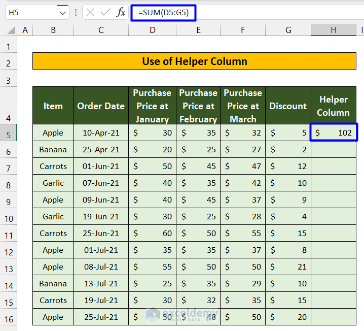
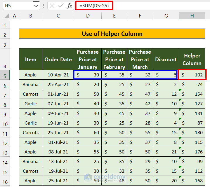
- We have added all the values in the first row. Use the Fill Handle to auto-fill the rest of the cells.
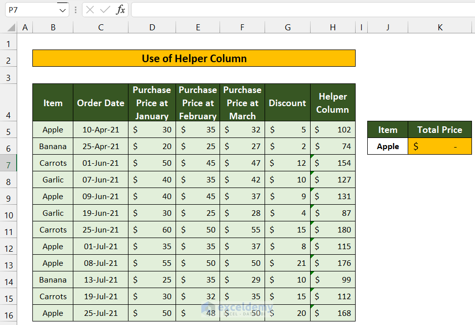
- We now have the helper column, use the criteria in cell J7 to evaluate the total price for Apple by applying the SUMIF function.
- In cell K7, enter the following formula.
=SUMIF(B5:B16,$J$6,H5:H16)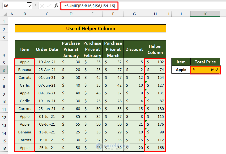
This method is only applicable when we can add an additional column.
Read More: SUMIF Across Multiple Sheets in Excel
Method 2 – Applying the SUM Function to SUMIF with Multiple Ranges
Steps:
- Enter the following formula in cell K6 and press Enter.
=SUM(SUMIF(B5:B16,J6,D5:D16),SUMIF(B5:B16,J6,E5:E16),SUMIF(B5:B16,J6,F5:F16),SUMIF(B5:B16,J6,G5:G16))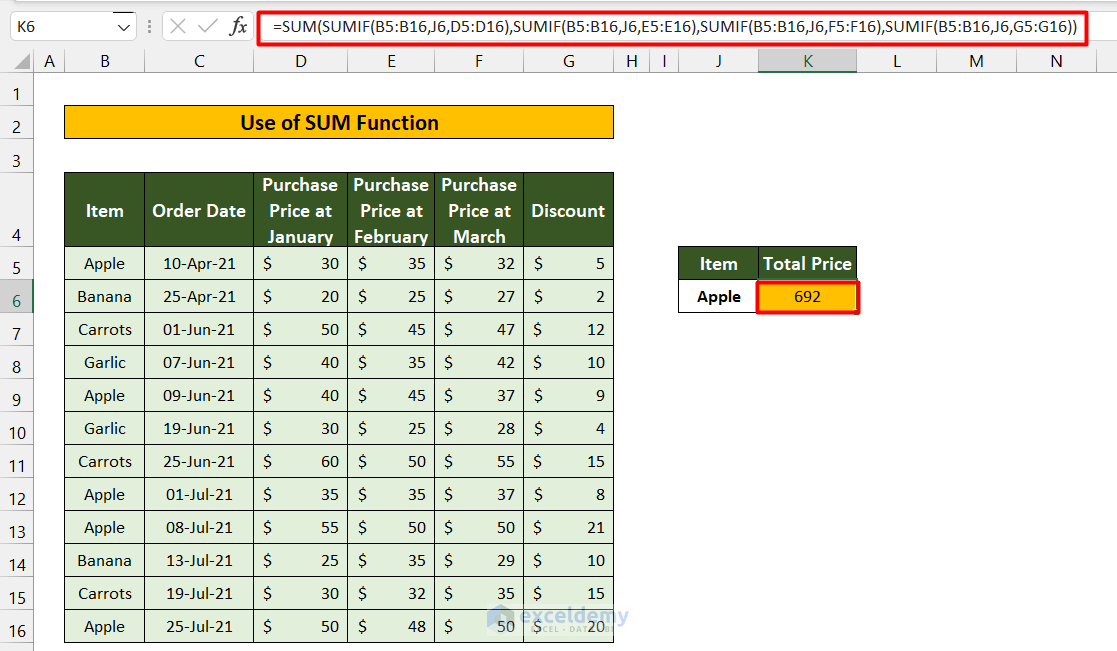
How Does the Formula Work?
- SUMIF(B5:B16,J6,D5:D16)
This part sums up the total price of Apple (J6) by looking up the criteria in the B5:B16 range for the month of January (D5:D16).
- SUMIF(B5:B16,J6,E5:E16)
It sums up the total price of Apple (J6) by looking up the criteria in the B5:B16 range for the month of February (E5:E16).
- SUMIF(B5:B16,J6,F5:F16)
This part sums up the total price of Apple (J6) by looking up the criteria in the B5:B16 range for the month of March (F5:F16).
- SUMIF(B5:B16,J6,G5:G16)
It sums up the total price of Apple (J6) by looking up the criteria in the B5:B16 range for the Discount column (G5:G16).
- SUM(SUMIF(B5:B16,J6,D5:D16),SUMIF(B5:B16,J6,E5:E16),SUMIF(B5:B16,J6,F5:F16),SUMIF(B5:B16,J6,G5:G16))
It sums up all four results obtained by the above 4 functions.
Method 3 – SUMIF with Multiple Ranges Using Addition Operator
Steps:
- Enter the following formula in cell K6 and press Enter.
=SUMIF(B5:B16,J6,D5:D16)+SUMIF(B5:B16,J6,E5:E16)+SUMIF(B5:B16,J6,F5:F16)+SUMIF(B5:B16,J6,G5:G16))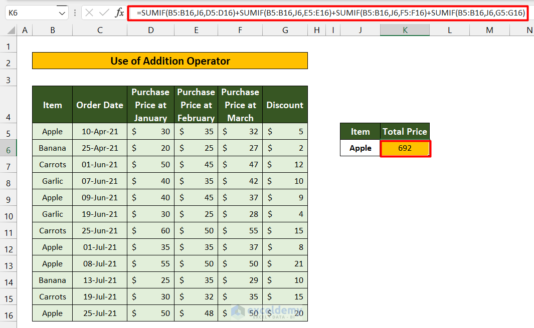
How Does the Formula Work?
- SUMIF(B5:B16,J6,D5:D16)
It sums up the total price of Apple (J6) by looking up the criteria in the B5:B16 range for the month of January (D5:D16).
- SUMIF(B5:B16,J6,E5:E16)
This part sums up the total price of Apple (J6) by looking up the criteria in the B5:B16 range for the month of February (E5:E16).
- SUMIF(B5:B16,J6,F5:F16)
This part sums up the total price of Apple (J6) by looking up the criteria in the B5:B16 range for the month of March (F5:F16).
- SUMIF(B5:B16,J6,G5:G16)
Sums up the total price of Apple (J6) by looking up the criteria in the B5:B16 range for the Discount column (G5:G16).
- SUMIF(B5:B16,J6,D5:D16)+SUMIF(B5:B16,J6,E5:E16)+SUMIF(B5:B16,J6,F5:F16)+SUMIF(B5:B16,J6,G5:G16))
It sums up all four results obtained by the above 4 functions.
Read More: How to Sum Based on Column and Row Criteria in Excel
Things to Remember
- Use the 1st method when you can add an additional column.
- Use the 2nd and 3rd methods when you have a small number of ranges to sum.
Download Practice Workbook
Related Articles
- SUMIF with Multiple Criteria in Different Columns in Excel
- How to SUMIF for Multiple Criteria Across Different Sheet in Excel
<< Go Back to SUMIF Multiple Criteria | Excel SUMIF Function | Excel Functions | Learn Excel
Get FREE Advanced Excel Exercises with Solutions!

