How to Prepare a Vacation Budget in Excel (with Easy Steps)

In this article, you will learn about three quick steps on how to create a vacation budget in Excel. We will be using the Microsoft 365 version; however, you can use any version of Microsoft Excel and follow this tutorial.

Step-by-Step Procedures to Prepare a Vacation Budget in Excel

There are three easy steps to create a vacation budget in Excel. Firstly, we will set up the dataset. Secondly, we will enter the estimated and actual values. Lastly, we will create a pie chart to visualize the category-wise expense distribution.

Step 1: Setting Up Dataset

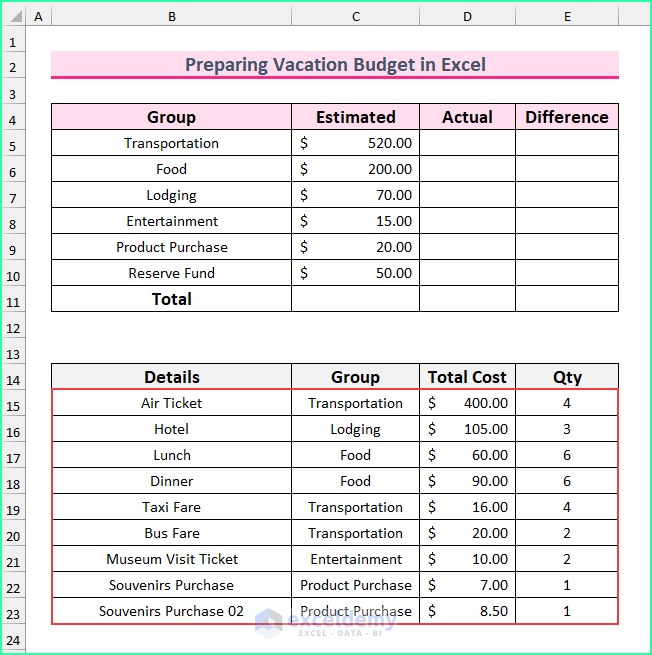
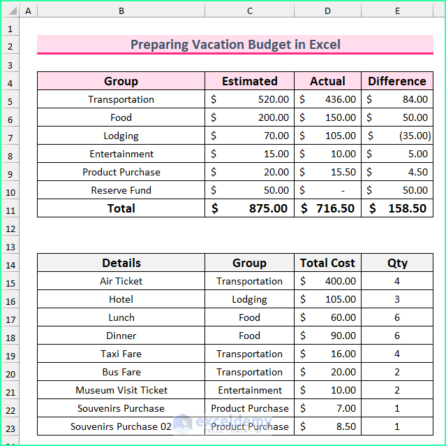
We will enter the required columns and fields in this first step. There will be two tables and four columns each. The first table, which is the main budget table, consists of “Group”, “Estimated”, “Actual”, and “Difference” columns. Then, we have the helper table to show the detailed expenses for the groups in the main table.

Firstly, type all the following fields in the Excel sheet.

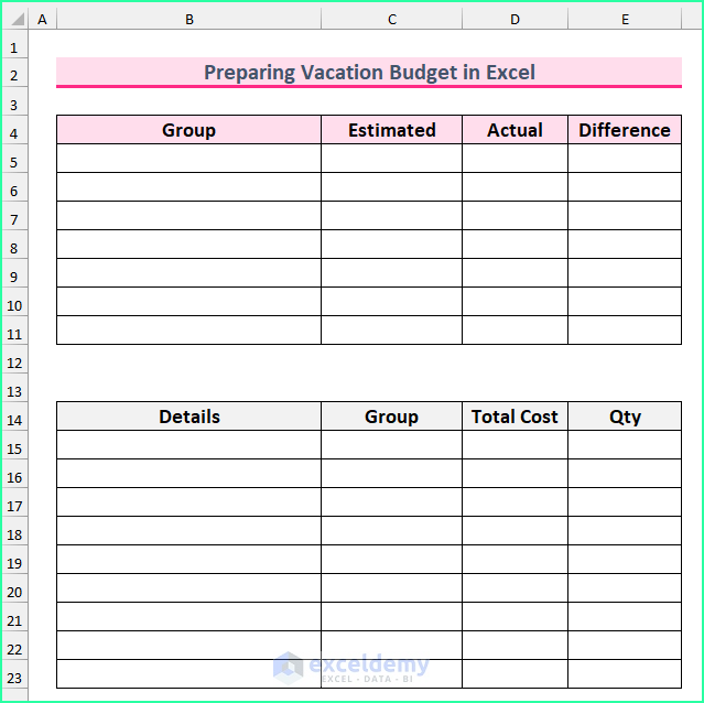
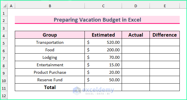
Secondly, type the classification of the expense in the “Group” column.
Thirdly, type all the estimated values in the next column.

Lastly, type the breakdowns of the expense groups in the lower table.

Step 2: Calculating the Values

We will use the SUMIF and SUM functions in the second step to calculate the actual expenses and total value, respectively. Moreover, we will use the Fill Handle to fill the formulas into the relevant cells. Additionally, we will also use the fixed cell reference in our first formula.

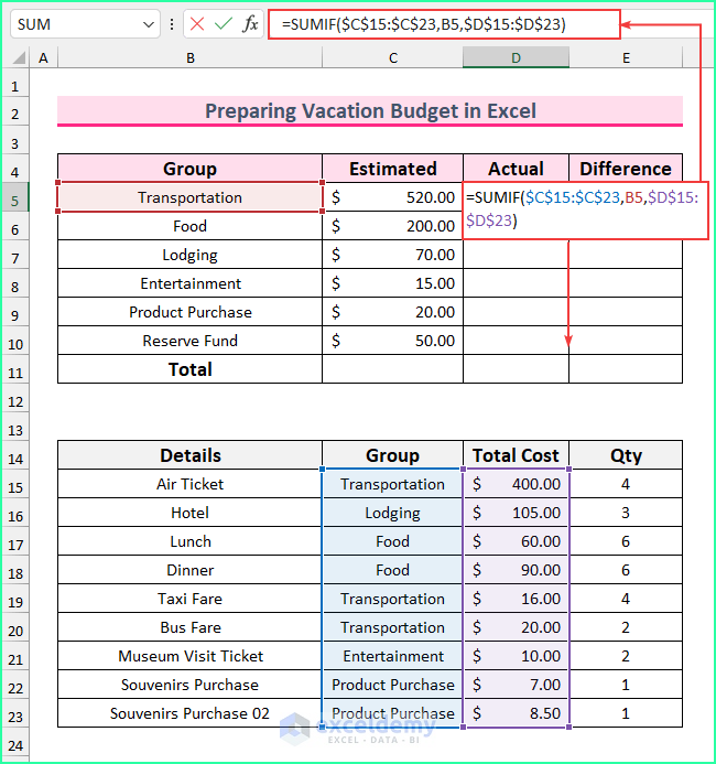
To begin with, type the following formula in cell D5 and AutoFill the formula into the rest of the cells downward.

=SUMIF($C$15:$C$23,B5,$D$15:$D$23)

Formula Breakdown

This function returns the total value from a range of cells for a condition in Excel.
Firstly, we are applying the condition to the cell range C15:C23.
Secondly, the condition is that the above range needs to equal the value from cell B5. This means we are aggregating the values from the group “Transportation”.
Lastly, we have set the cell range D15:D23 as the sum range.

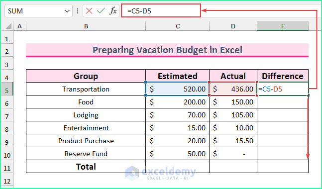
Next, type the following formula to return the difference between the forecasted and actual values.

=C5-D5

Finally, press ALT+= to calculate the total values. Then, drag the Fill Handle to the right side to fill that formula.

=SUM(C5:C10)

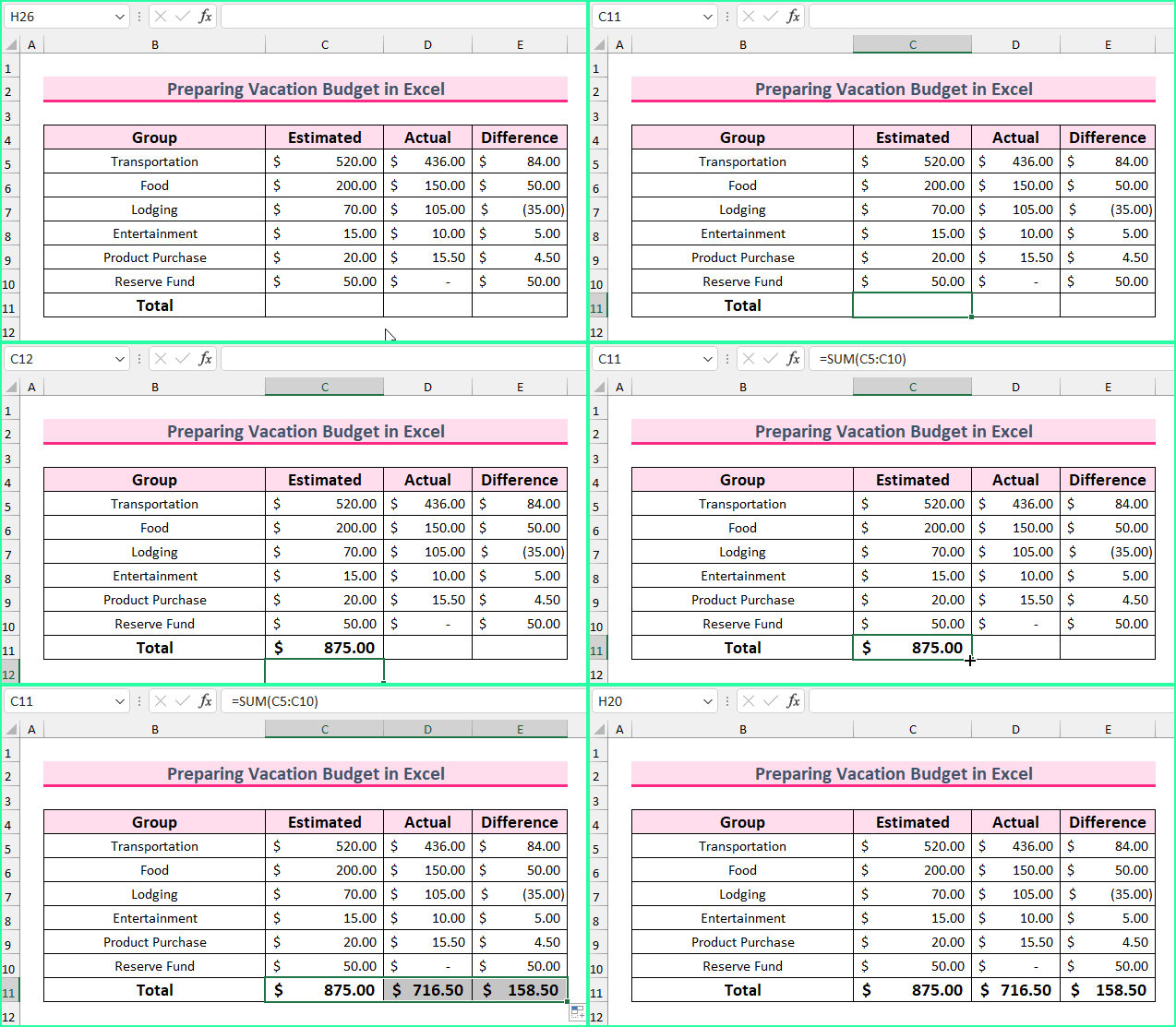
This will complete our vacation budget and the final output will look similar to this.

Step 3: Creating Doughnut Chart

In the last step, we will create a doughnut chart to visualize the actual expense breakdown. We will select the cell range first. After that, we will bring up the Insert Chart window. Finally, we will select the doughnut chart from the pie chart section in Excel. Without further ado, allow us to demonstrate how to carry out these.

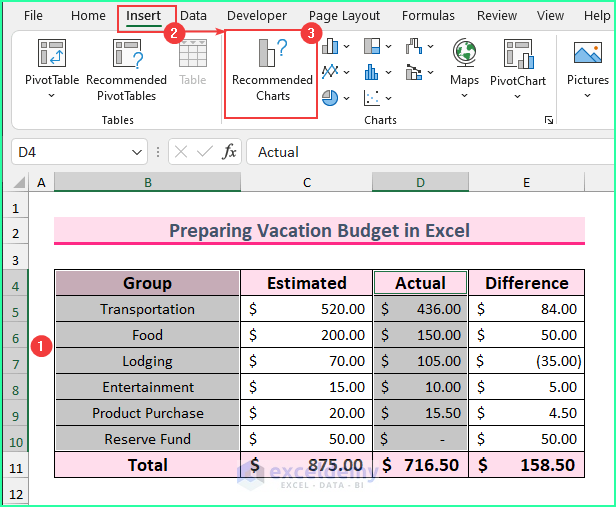
Firstly, select the cell range B4:B10 and D4:D10 by holding the CTRL key and dragging with the mouse.
Secondly, from the Insert tab, select Recommended Charts.

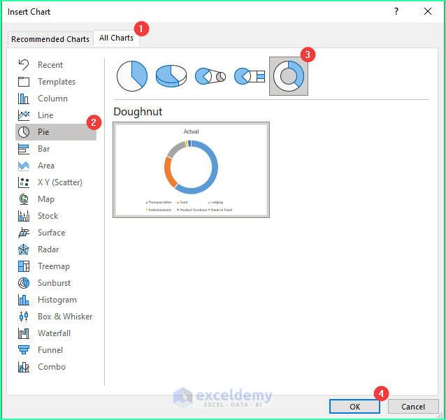
Then, the Insert Chart window will pop up.
Next, from the All Charts tab, select Doughnut from the Pie chart section and press OK.

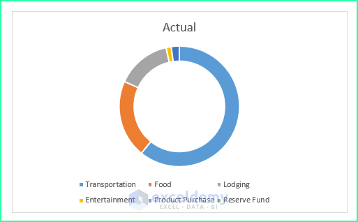
Therefore, a basic doughnut chart will appear.

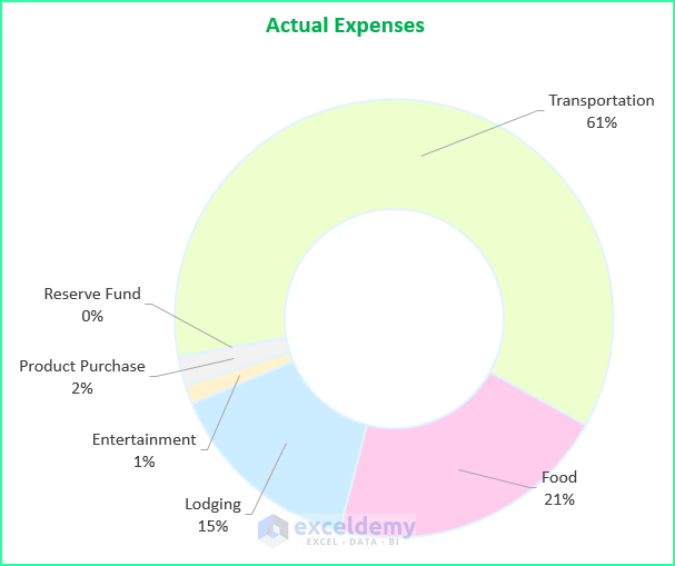
Now, after a few modifications, the doughnut chart will look better. We can see that most of the actual expenses are spent on transportation.

Road Trip Budget Template

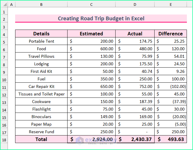
Now, we will show you quick steps on how to create a road trip budget template in Excel. This process is similar to the vacation budget template. Firstly, we will prepare the relevant details for the road trip budget. Then, we will input the expected and actual expense amounts. Lastly, we will deduct these values to return the difference between them.

Steps:

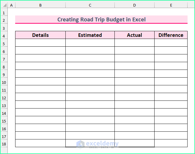
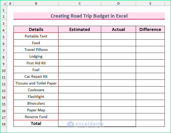
Firstly, type the following fields for data input.

Then, type the details of the activities in column B.

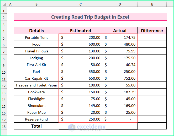
After that, type the estimated and the actual values in that road trip budget template.

Next, select the cell range E5:E17 and type the following formula.

=C5-D5

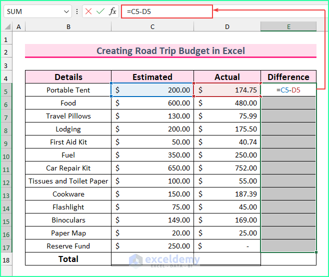
Then, press CTRL+ENTER.
Afterward, type another formula in cell C18 and fill that formula into the next two cells.

=SUM(C5:C17)

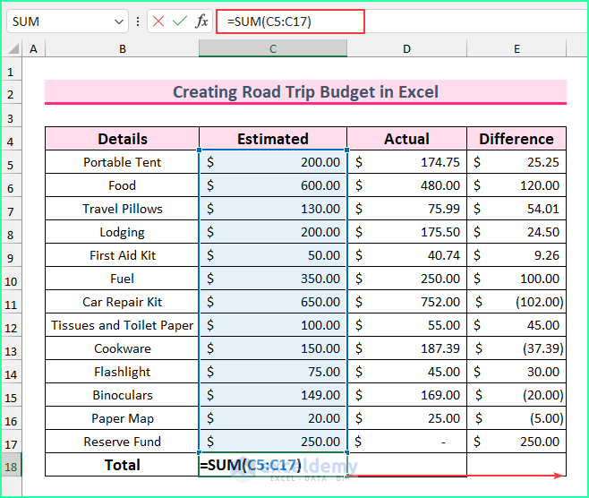
After doing all of the above steps, it will complete the road trip budget template in Excel.

Download Practice Workbook

You can download the Excel file from the link below.

Creating Vacation Budget.xlsx

Conclusion

We have shown you quick steps on how to prepare a vacation budget in Excel. If you face any problems regarding these methods or have any feedback for me, feel free to comment below. However, remember that our website implements comment moderation. Therefore, your comments may not be instantly visible. So, have a little bit of patience, and we will solve your query as soon as possible.

Thanks for reading, keep excelling!