Step 1 – Setting Up the Dataset
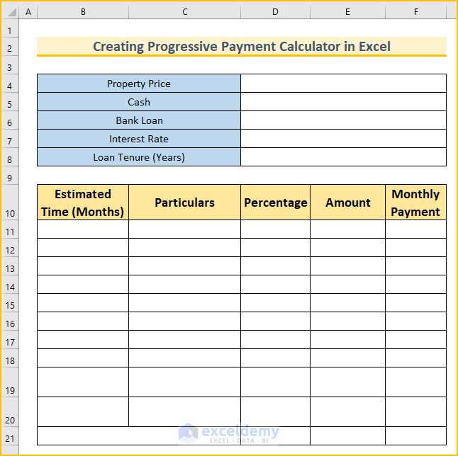
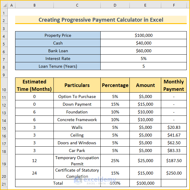
- Create the following fields.

- Insert a table with five columns: “Estimated Time (Months),” “Particulars,” “Percentage,” “Amount,” and “Monthly Payment.”
Step 2 – Calculating the Progressive Payment
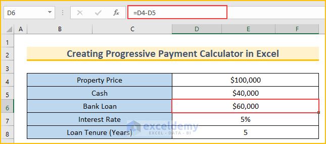
- Type in the property price, cash amount, interest rate, and loan tenure.
- Insert the following formula to find the bank loan amount.
=D4-D5
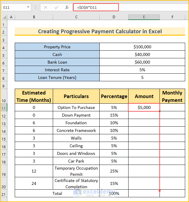
- Type the values for the first three columns.
- Use this formula in cell E11 and drag the Fill Handle down to fill the column.
=$D$4*D11
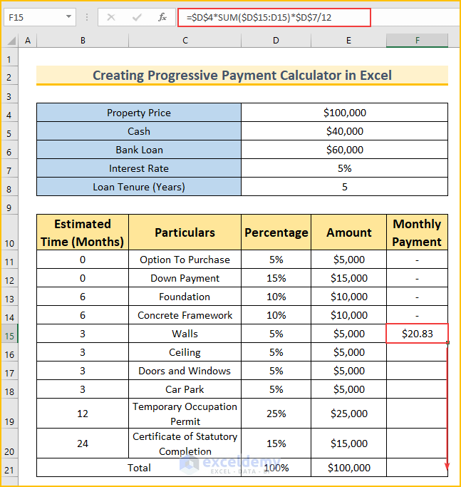
- Insert this formula to calculate the monthly payment.
=$D$4*SUM($D$15:D15)*$D$7/12
Formula Breakdown
- We are using a dynamic range inside the SUM function. This is the main step for finding the progressive payment.
- The interest rate is provided per annum. We are dividing it by 12 to find the monthly interest rate.
- Our cash amount is $40,000 and we do not need to pay anything until this value depletes. Calculate it from row 15. You should modify this to fulfill your requirements.
- We multiply the above two values by the property price to return the monthly payment.
- AutoFill the formula to finish creating the progressive payment calculator in Excel.
Download the Practice Workbook
Related Articles
- How to Create Line of Credit Payment Calculator in Excel
- How to Make HELOC Payment Calculator Using Principal and Interest in Excel
- How to Make HELOC Payment Calculator in Excel
<< Go Back to Payment Calculator | Finance Template | Excel Templates
Get FREE Advanced Excel Exercises with Solutions!

