How to Prepare Charitable Trust Balance Sheet Format in Excel

Running a charitable trust organization? Looking to create a balance sheet for your organization? Hey…hold on! Stick to this article. Here, I am going to show you how to create a charitable trust balance sheet format in Excel. At the end of the article, you will be able to create one by yourself.

Charitable Trust Balance Sheet

A charitable trust is a tax-exempt non-profit charitable organization. It allows an individual to donate assets to this organization and also provides certain tax benefits that personnel is owed to the government. It is a tax-efficient way to donate to charities or non-profit organizations according to your choice. This kind of trust is generally irrevocable. So you can’t change your decision or undo the trust if your situation is not in hand and you can’t refund the money donated to the trust.

A balance sheet is one of the three most important financial statements. This statement creates a report of the company’s assets, liabilities, shareholder equity, etc over a certain period of time. So, a charitable trust balance sheet can be created by using the factors that are used to report the situation of a charitable trust organization.

Stepwise Guideline to Create Charitable Trust Balance Sheet Format in Excel

Let’s say, we are dealing with a charitable trust organization XYZ Limited. We want to create a balance sheet for this organization.

In this section, you will find some useful and handy steps to create a charitable trust balance sheet format in Excel. I will demonstrate them with proper illustrations here. Let’s check them now!

⏩ Step 1: Insert Balance Sheet Components

The first and foremost task is to deal with the components of the charitable trust organization.

First of all, create a table and add proper headings to the table for your worksheet in Excel. The main category we have assigned here:

Liabilities
Properties & Assets

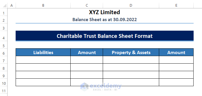
Then, add components to the corresponding type of category. The components we have set for Liabilities are

Capital Account
Loans
Current Liabilities
Income and Expenditure

For Property & Assets, the components are chosen as:

Fixed Assets
Investments
Current Assets
Income Outstanding

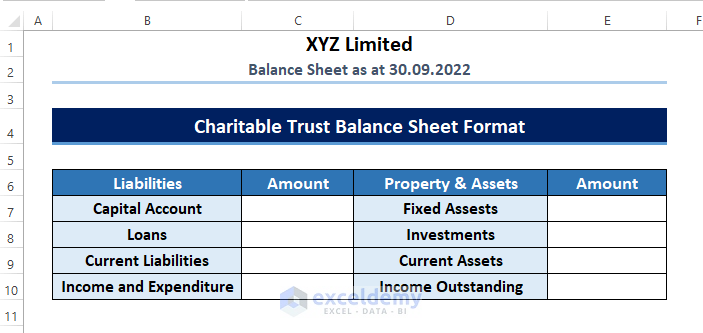
After that, assign sub-factors under each type of component as stated in the screenshot below.

⏩ Step 2: Input Values for the Components

After completing the first step of creating your balance sheet in the Excel worksheet, it’s time to input values for the sub-factors of each type of component under the category level. Let’s deal with the category of Liabilities first.

The first component under the category of Liabilities is the Capital Account. The factors encountered here are Reserve and Surplus & Share Capital. Input values for these two types of factors.

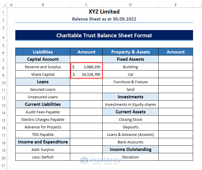
💬Note: Format the cells to Accounting or Currency for inputting the amounts.

Now, summing these two components will result in the total amount of the Capital Account. The SUM function is used in Excel to sum up a number of values. So, in order to find out the total Capital Account, select a cell and type the following formula in the selected cell.

=SUM(C8:C9)

Here,

C8 = Amount of Reserve and Surplus
C9 = Amount of Share Capital

Now, press ENTER, and your cells will get you the total amount of the Capital Account.

After that, input values for the other types of factors under each component (i.e. Loans & Current Liabilities) and calculate the total amount for the components.

Here, one thing is noticeable: in the case of Income and Expenditure, you should subtract the Deficit from the Surplus.

=C19-C20

Here,

C19 = Amount of Surplus
C20 = Amount of Deficit

⏩ Step 3: Calculate Total Amount of Liabilities

After assigning the factors and finding the encountering amount for each of the factors under the category of Liabilities, you have to calculate the total amount of Liabilities for your balance sheet.

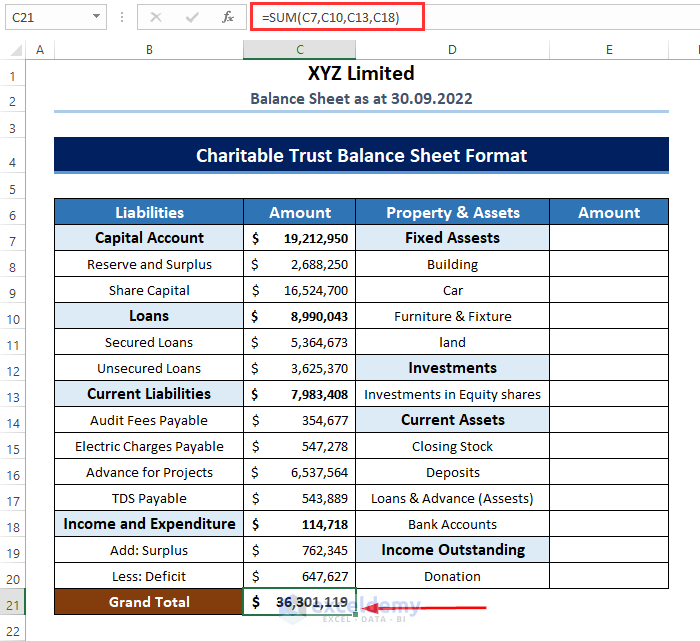
Now, in order to calculate the grand total of the Liabilities, apply the following formula.

=SUM(C7,C10,C13,C18)

Here,

C7 = Total Amount of Capital Account
C10 = Total Amount of Loans
C13 = Total Amount of Current Liabilities
C18 = Total Amount of Income and Expenditure

⏩ Step 4: Determine Total Amount of Property and Assets

There are a few tasks still to be done. Now, work on the category: Property and Assets.

Here, repeat the task of inputting values to the sub-factors under this category.

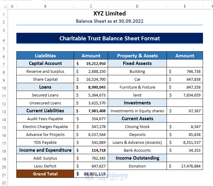
Now, determine the total amount of the components: Fixed Assets, Investments, Currents Assets, and Income Outstanding.

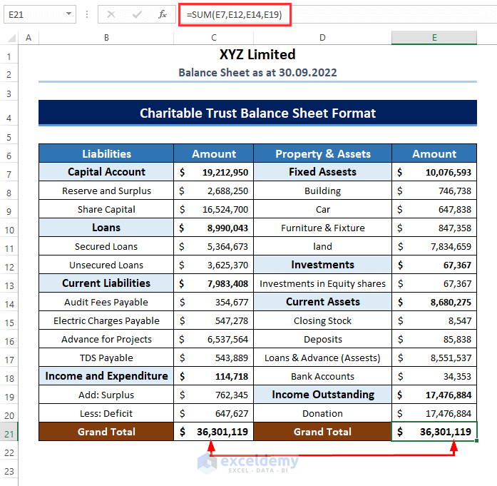
Now, apply the following formula to find out the grand total of Property & Assets.

=SUM(E7,E12,E14,E19)

Here,

E7 = Total Amount of Fixed Assets
E12 = Total Amount of Investments
E14 = Total Amount of Current Assets
E19 = Total Amount of Income Outstanding

💬Note: When the Property and Liabilities are the same then it’s in a balanced state.

Download Practice Workbook

You can download the practice book from the link below.

Charitable Trust Balance Sheet Format.xlsx

Conclusion

In this article, I have tried to show you some methods to create a charitable trust balance sheet in Excel. I hope this article has shed some light on your way. If you have better techniques, questions, or feedback regarding this article, please don’t forget to share them in the comment box. For more queries, kindly visit our website. Stay connected to get more articles.

<< Go Back to Balance Sheet | Finance Template | Excel Templates

Get FREE Advanced Excel Exercises with Solutions!