How to Change Comma in Excel to Indian Style (with Easy Steps)

Similar to how India uses the 2, 2, 3 system of number value accounting for lakhs, the U.S. uses 3, 3, 3 for millions. We will show you how to change the comma separator in Excel to the Indian style. Let’s suppose we have a sample data set for profits.

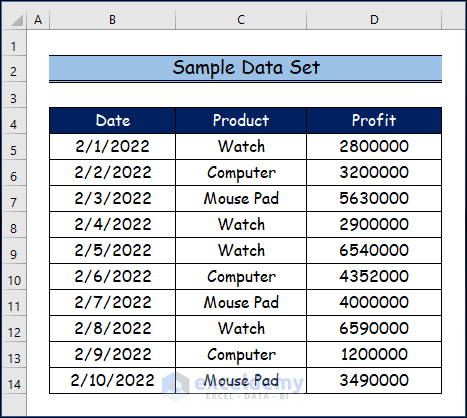
Step 1 – Creating the Data Set with Proper Parameters

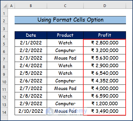
Here is our sample data set, where we’ve manually put the values. You will see the profit values are in the general usual format in US dollars in millions. We want to change this format to the Indian style in lakhs.

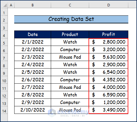
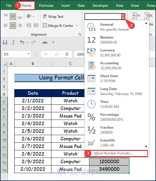
Step 2 – Using the Format Cells Option

• Go to the Home tab.
• Click the arrow on the drop-down that shows the Number group.
• Select the More Number Formats… option.

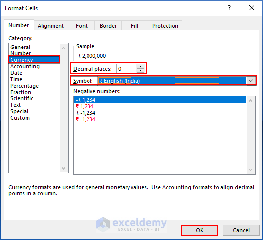
• The Format Cells box will open.
• Go to the Currency option.
• Keep decimal places at 0 and select the English (India) symbol.
• Click OK.

• This changes the value to represent rupees.

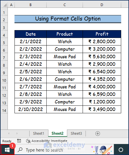
• Click on the Start button.

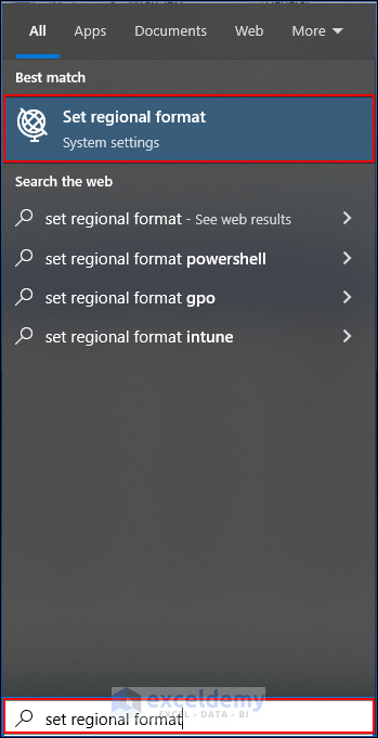
• Type Set Regional Format and click on the first result.

• Change the Regional Format to English (India).

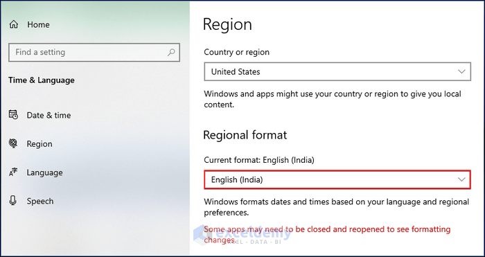
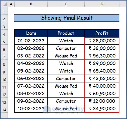
Step 3 – Showing Final Result

• Here’s how the table will be converted after setting the regional style to India.

Read More: How to Change Comma Style in Excel

Download Practice Workbook

You may download the following Excel workbook for practice.

Related Articles

• How to Put Comma After 2 Digits in Excel
• How to Put Comma after 3 Digits in Excel
• How to Put Comma After 5 Digits in Excel
• How to Convert Column to Row with Comma in Excel
• How to Put Comma in Numbers in Excel
• How to Change Semicolon to Comma in Excel
• [Fixed!] Style Comma Not Found in Excel

<< Go Back to How to Add Comma in Excel | Concatenate Excel | Learn Excel