Method 1 – Unprotecting Worksheet
Step 01: Pasting Link in a Protected Worksheet
See what happens when we try to paste a link into a protected worksheet.
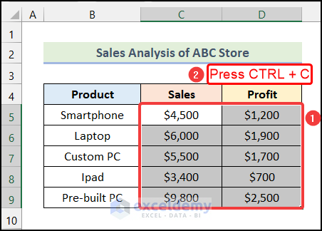
- Select the cells of the Sales and the Profit columns and press the keyboard shortcut CTRL + C to copy the cells.
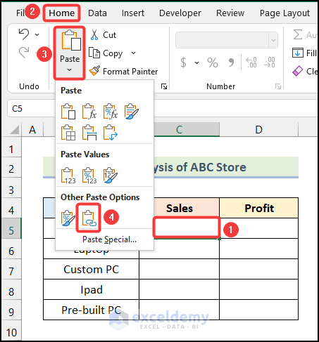
- Go to the protected worksheet and select cell C5.
- Go to the Home tab from the ribbon.
- Choose the Paste option from the Clipboard group.
- Select the Paste Link option from the drop-down.
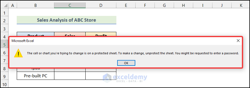
You will have the following error message as shown in the following image.
Step 02: Unprotecting the Worksheet
- Right-click on the worksheet name and select the Unprotect Sheet option.
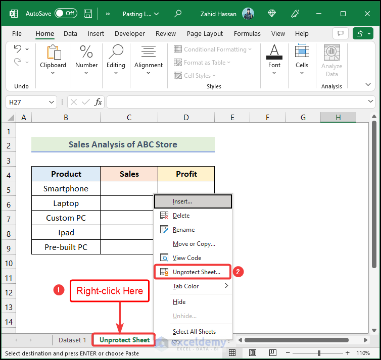
The Unprotect Sheet dialogue box will open on your worksheet.
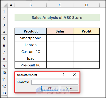
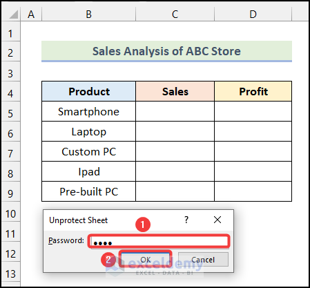
- In the Unprotect Sheet dialogue box, enter your password.
- Click OK, and your worksheet will be unprotected.
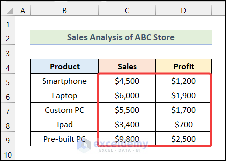
- Follow the steps mentioned in step 01 of this method and you can paste the copied cells as a link.
Method 2 – Resetting Toolbar
Steps:
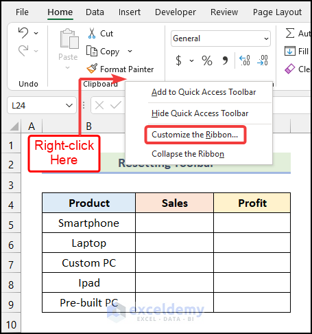
- Right-click on any portion of the empty space on the ribbon.
- Select the Customize the Ribbon option.
The Excel Options dialogue box will open on your worksheet.
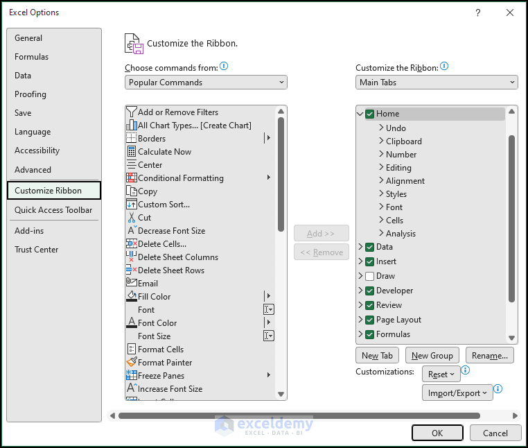
Note: You can also use the keyboard shortcut ALT + F + T to directly open the Excel Options dialogue box from your worksheet.
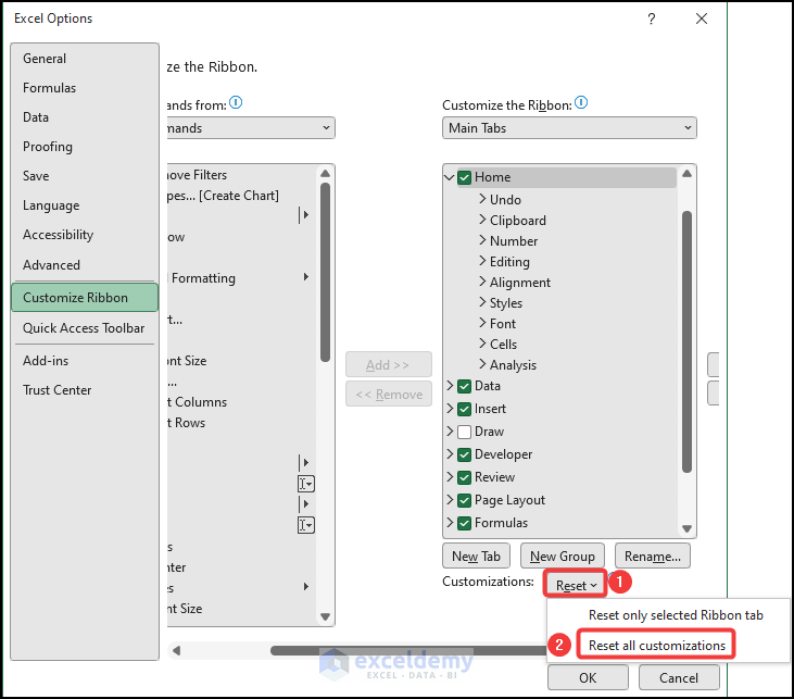
- Click on the Reset option, as marked in the following picture.
- Choose the Reset all customizations option from the drop-down.
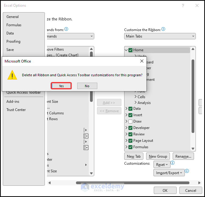
- Click OK in the Microsoft Office dialogue box.
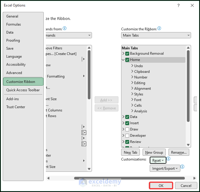
- Click OK in the Excel Options dialogue box.
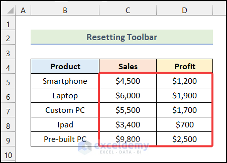
- You can use the steps outlined in step 01 of the 1st method and you will have the following outputs as shown in the image below.
Method 3 – Applying Excel Formula
Steps:
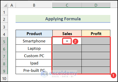
- Select the cells where you want to Paste Link.
- In cell C5 type in = to start the formula.
- Go to the worksheet with the original data. In this case, we selected Dataset 1.
- Choose the cells under the Sales and the Profit columns.
- Press the keyboard shortcut SHIFT + ENTER to apply the formula.
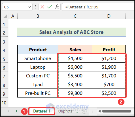
Note: Here, we used SHIFT + ENTER instead of ENTER as it’s an array formula. However, you don’t need to press SHIFT if you’re a Microsoft 365 user.
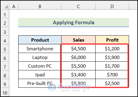
You will have the following outputs, as demonstrated in the following picture.
What to Do When Paste Special is Not Working in Excel
Method 1 – Using Excel Options Feature
Steps:
- Go to the File tab from Ribbon.
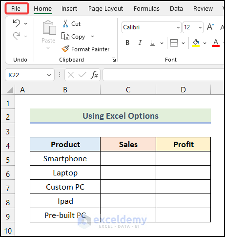
- Click on Options as marked in the following image.
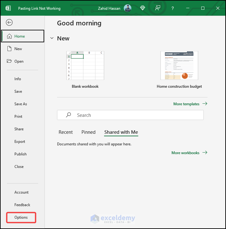
- In the Excel Options dialogue box, select the Advanced tab.
- Make sure to check the field of the Show Paste Options button when content is pasted in the Cut, copy, and paste section.
- Click on OK.
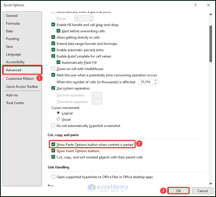
This should make the Paste Special option visible in your worksheet.
Method 2 – Opening Excel in Safe Mode
Steps:
- Go to the search bar of windows and type in Excel.
- Press and hold the CTRL key and click on the Excel App.
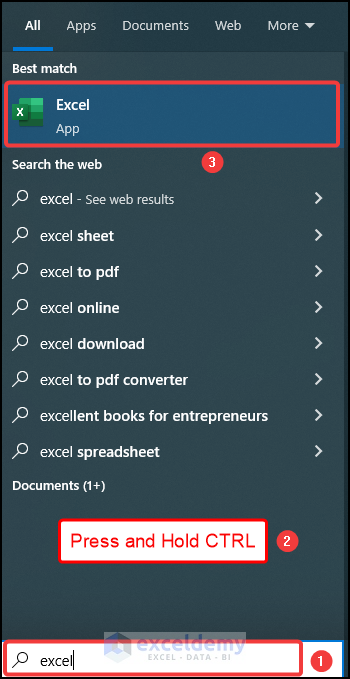
- Click Yes in the following pop-up window.

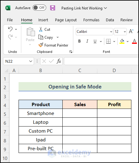
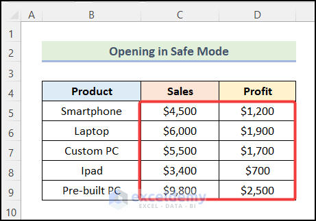
Excel will start in Safe Mode, as shown in the following picture.
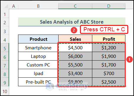
- Select the cells and press the keyboard shortcut CTRL + C to copy the cells you want to paste into your target worksheet.
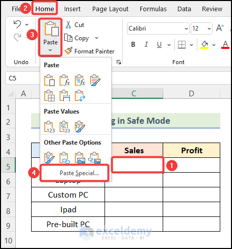
- Go to your target worksheet and select the cells where you want to paste.
- Go to the Home tab from the ribbon.
- Choose the Paste option from the Clipboard group.
- You will be able to see the Paste Special option in the drop-down.
- Click on the Paste Special option.
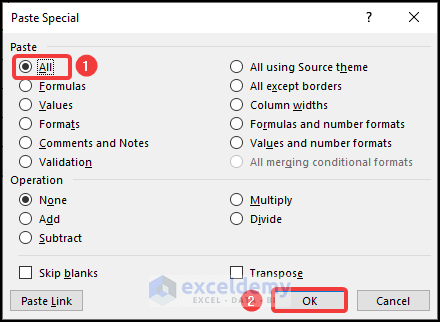
- In the Paste Special dialogue box, choose the All option under the Paste section.
- Click OK.
Your copied cells will be pasted, as demonstrated in the following picture.
Download Practice Workbook
Related Articles
- [Solved] Excel Copy Paste Loses Formatting
- [Fixed!] Cannot Copy Merged Cells in Excel
- How to Copy Number Not Formula in Excel
- [Fixed!] Copy and Paste Not Working Between Workbooks in Excel
- [Fixed!]: Microsoft Excel Cannot Paste the Data as Picture
- [Fixed!] CTRL C Not Working in Excel
<< Go Back to Copy-Paste Not Working | Copy Paste in Excel | Learn Excel
Get FREE Advanced Excel Exercises with Solutions!

