Method 1 – Generate a Sequence of Workdays
Generate a sequence of workdays using the WORKDAY function. The following are the steps to do that.
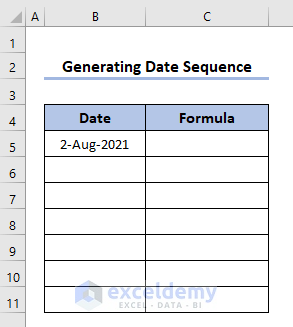
- Insert a date in cell B5. Generate the sequence of working days from this date.
- The generic formula for our task will be
=WORKDAY(date,1)
- A consecutive sequence we are going to use 1 in the days field.
- Write the formula in Excel.
=WORKDAY(B5,1)- Using the formula we found the next working date. We used Cell Reference in the formula.
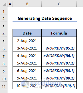
- Keep copying the formula to find the sequence you want.
- Generate the weekdays of the working days using the following formula.
=TEXT(WEEKDAY(B5,1),"ddddd")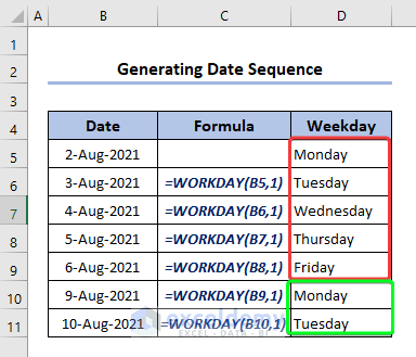
- The WORKDAY function generally identifies Saturday and Sunday as weekends (the US form). It returned Monday to Friday and then repeated.
Method 2 – Generate Workdays After Given Days
We can generate workdays from a date after any specific number of days.
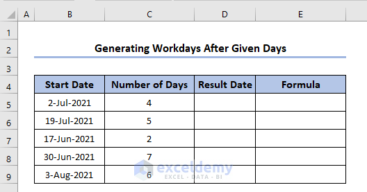
- We have two inputs, start date, and number of days, our formula will be:
- Write the formula in Excel.
=WORKDAY(B5,C5)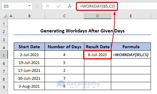
- The formula uses Cell Reference. See, our start date was 02-Jul-2021, and the number of days was 4. The result is 08-Jul-2021.
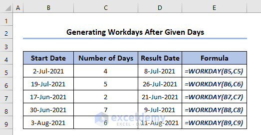
- See the difference between the two dates, they are not 4. As the name suggests, WORKDAY only produces working days of a week; it discards Saturday and Sunday from working days.
- Copy the formula for the rest of the values.
Method 3 – Generate Next Working Days
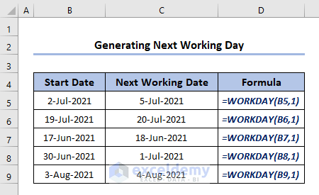
Produce the next working day from a date using the WORKDAY function.
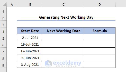
- Find the next date we need to use 1 in our days field.
- Write the formula in Excel.
=WORKDAY(B5,1)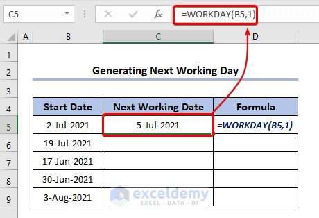
- We found the next workdays from the provided date.
- Do the same for the rest of the values.
Method 4 – Find Working Days in Excel Excluding Weekends and Holidays
- We introduced a list of holidays to our dataset. The holidays are listed in B12:B14.
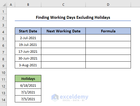
- The derived date WORKDAY(start_date,1) matches in the holidays list that day will be eliminated from the working day and search for another workday.
- The formula will be something like below
- Write the formula in Excel.
=WORKDAY(B5,7,$B$12:$B$14)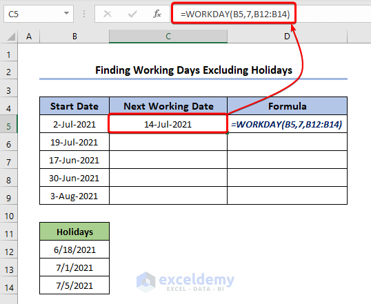
- We found the next working date. Using a similar dataset in the previous section, you can see that the result has been changed.
- Earlier for 02-07-2021, our next working day was 05-07-2021, but now 05-07-2021 is the Holidays, and that’s why it was not counted as a workday. We have found 06-07-2021 as the next working day after 02-07-2021.
- Do the same for the rest of the values.
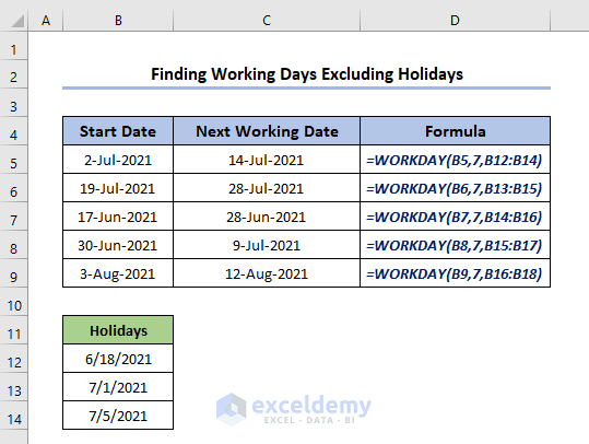
- You can see Holidays have an impact on the next working date.
- Last two examples we have derived the very next working day, if you need after a certain amount just change the values of the days parameter. (In the above image we found the 7th working day)
Method 5 – Check Whether a Day Is a Holiday or a Working Day
Check whether a day is a holiday or a working day using the WORKDAY function.
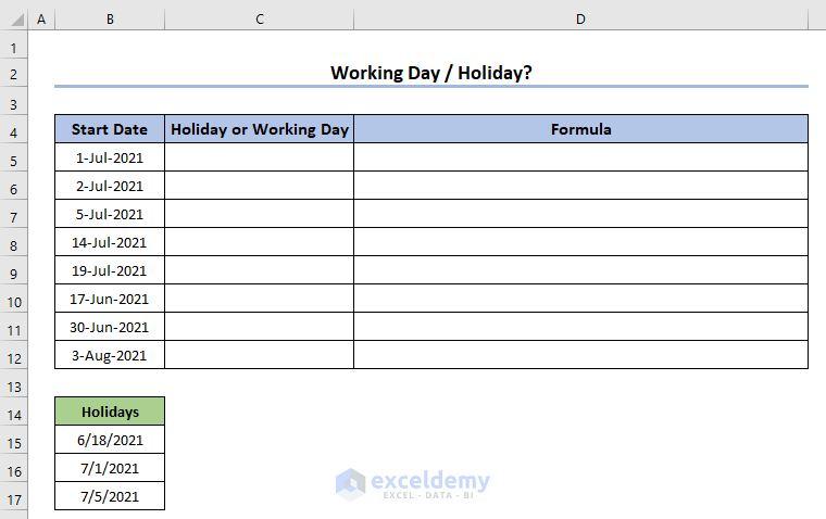
- Check we need to apply a condition statement. The IF function will be helpful for condition checks.
- Our formula will be
=IF(WORKDAY(B5-1,1,$B$15:$B$17)=B5,"Working Day","Holiday")- Using date-1 in the start_day field of WORKDAY so that the function can eventually return that date.
- We checked the derived date from our given date. If they match we set it to return Working Day, Holiday otherwise.
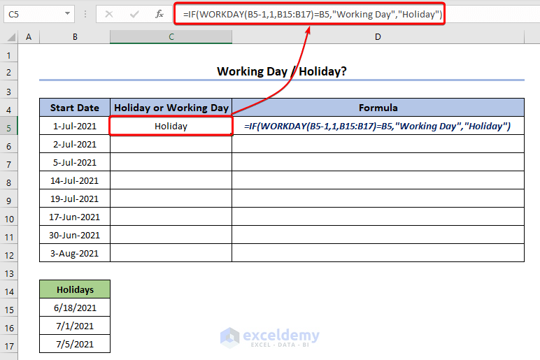
- 01-07-2021 was listed in the Holidays and our formula identified it as a holiday. Do the same for the rest of the values.
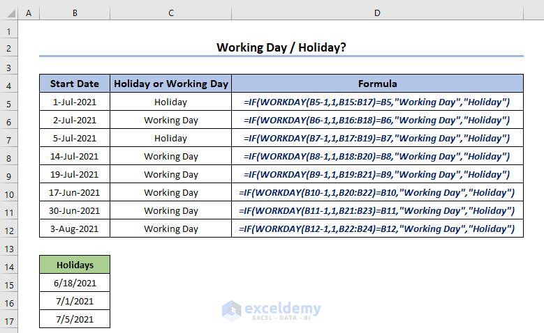
We instructed you to write the formula just to perform the practice. The more you practice the more skillful you will be.
Method 6 – Excel WORKDAY Function with Hours
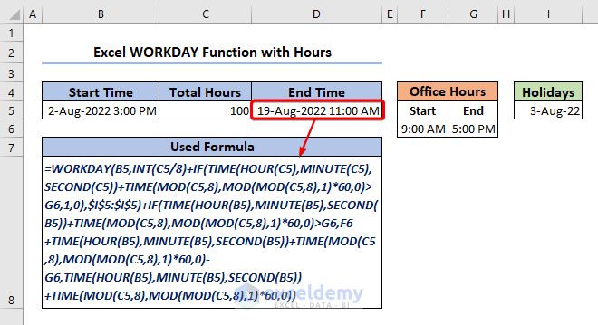
- Specify Start Time, Total Hours, Office Hours, and Holidays (if any). We have specified all these in the following dataset.
- Apply the following formula in the End Time cell:
=WORKDAY(B5,INT(C5/8)+IF(TIME(HOUR(C5),MINUTE(C5),SECOND(C5))+TIME(MOD(C5,8),MOD(MOD(C5,8),1)*60,0)>
G6,1,0),$I$5:$I$5)+IF(TIME(HOUR(B5),MINUTE(B5),SECOND(B5))+TIME(MOD(C5,8),MOD(MOD(C5,8),1)*60,0)>G6,F6
+TIME(HOUR(B5),MINUTE(B5),SECOND(B5))+TIME(MOD(C5,8),MOD(MOD(C5,8),1)*60,0)-G6,TIME(HOUR(B5),MINUTE(B5),SECOND(B5))
+TIME(MOD(C5,8),MOD(MOD(C5,8),1)*60,0))
Credit goes to extendoffice for this formula.
- Get to see the result immediately.
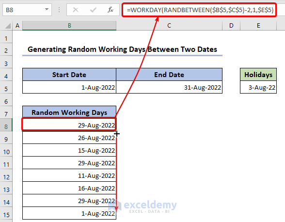
Method 7 – Combine RANDBETWEEN Function with WORKDAY to Generate Random Working Days Between Two Days
- Use the following formula once to get a random working day.
=WORKDAY(RANDBETWEEN($B$5,$C$5)-2,1,$E$5)- Copy the formula.
Quick Notes
You need to keep several things in mind while using any function, so do for WORKDAY, here are some honorable mentions.
- Ways to Insert Dates in WORKDAY
You can insert dates in WORKDAY in various ways. Previously we have provided dates using Cell Reference.
♠ You can input your dates directly, as in the image below.
=WORKDAY("3-08-2021",1)
We have inserted the date. You might have understood the reason for using 1. Yes, we are aiming to produce the next day.
♠ You can input the date using the DATE function.
=WORKDAY(DATE(2021,3,8),7)
We have used DATE inside the WORKDAY function. This time we aim for the 7th working day from the given date.

♠ If you want to find the next ( or any other, change the day value) working day from the current day, feel free to use the TODAY function.
The TODAY function returns the present-day dynamically in Excel.
=WORKDAY(TODAY(),10)
We have inserted the TODAY function within WORKDAY and 10 in the day parameter. it returned our desired future work date (see the image below).

We are creating this article on 3 August 2021; the 10th working day from this day is 17 August 2021.
- Common Problems
♠ #VALUE! Error:
If you provide a value in the function which is not a valid date then this error will appear.
Insert a text string within WORKDAY.
To use Cell Reference we have written hello in a cell.
Insert the string in the WORKDAY function.
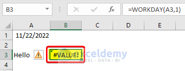
This will return a #VALUE! error. Since the string is not a valid date.
See another example. This time use a date.
Use the function for this date.
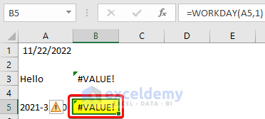
We have written the date in yyyy-dd-mm format. Which is not a valid date format in Excel in the US region. So, it returned the error.
♠ #NUM! Error:
This error occurs if the supplied start_date and/or the supplied days argument results in an invalid date.
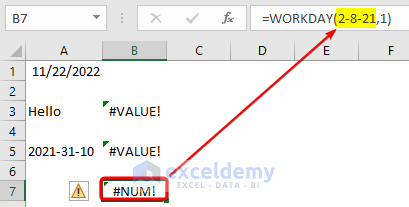
We have inserted 03-08-2021 in the function. The function cannot detect it properly and so returns an invalid date. The #NUM! error occurred.
Download Practice Workbook
You are welcome to download the practice workbook from the link below.
Excel WORKDAY Function: Knowledge Hub
- How to Find Last Business Day of Month in Excel
- How to Calculate Working Days Excluding Sundays in Excel
- How to Calculate Working Days in a Month in Excel
<< Go Back to Excel Functions | Learn Excel
Get FREE Advanced Excel Exercises with Solutions!


For referencing a data set for excluding holidays in the WORKDAY function, how do you keep the data reference correct when applying to a whole column (e.g. using ctrl+D)? In your example above, it would not work as you actually are only applying the full list of holidays for the first row; the formula is altered to be outside your data set for all the remaining cells (shifted one down), thus misses removing holidays. I’m having the same issue and need a fix!
Dear Annie
Thanks for visiting our blog and sharing an important fact! You are right that the holiday range reference shifts when you copy the formula. You need to use absolute references for the holiday range to fix the issue. Another improvement you can consider is not keeping the holiday list and start date or next working dates in the same column. Assume the start date and next working date data are in columns B and C; the holiday list is in column E.
Don’t worry! I have demonstrated an improved Excel file to overcome the situation. Please check the following:
Follow these steps:
Hopefully, you have found the solution you were looking for. I have attached the solution workbook as well. Good luck.
DOWNLOAD SOLUTION WORKBOOK
Regards
Lutfor Rahman Shimanto
ExcelDemy