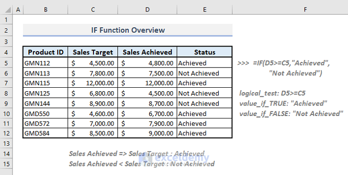
Here’s an overview of how the IF function can be used to put values into the Status column depending on the data in other cells.
Introduction to the IF Function

- Function Objective:
Checks whether a condition is met, and returns one value if TRUE, and another one if FALSE.
- Syntax:
=IF(logical_test, [value_if_true], [value_if_false])
- Arguments Explanation:
| Argument | Compulsory/Optional | Explanation |
|---|---|---|
| logical_test | Compulsory | Given condition for a cell or a range of cells. |
| [value_if_true] | Optional | Defined statement if the condition is met. |
| [value_if_false] | Optional | Defined statement if the condition is not met. |
- Logical Operators:
| Operator | Description |
|---|---|
| = | Equal to |
| <> | Not Equal to |
| > | Greater Than |
| >= | Greater Than or Equal to |
| < | Less Than |
| <= | Less Than or Equal to |
- Return Parameter:
Logical values- TRUE or FALSE if statements are not defined. If statements are defined, they’ll be shown as return values based on the conditions met or not.
How to Use IF Function in Excel: 8 Suitable Examples
Method 1 – Using the IF Function to Show Statements Based on a Logical Test
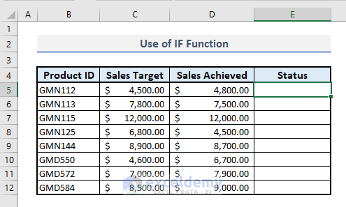
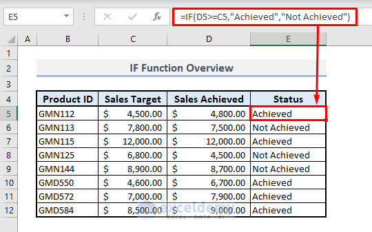
In our dataset, there are two columns containing the Sales Target and Sales Achieved for some products. We’ll check and show statements in Column E if the achieved sales have met the target or not.
Steps:
- In the output Cell E5, insert the following formula:
=IF(D5>=C5,"Achieved","Not Achieved")- Press Enter and use the Fill Handle to autofill the entire column.
Method 2 – Using the IF Function to Return Calculated Results
Steps:
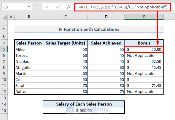
- Select Cell E5 and copy the following formula into it:
=IF(D5>=C5,$C$15*(D5-C5)/C5,"Not Applicable")- Press Enter and autofill the entire column.
- You’ll find the bonuses for those who have met the sales target, and the formula will return with the statement “Not Applicable” if target sales are not achieved.
Read More: How to Use MAX IF Function in Excel
Method 3 – Using Nested IF Functions in Excel
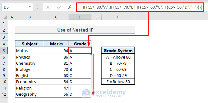
In the sample table, the first two columns consist of subject names and marks out of 100 for each one. Column F shows the grading system. We’ll find out the letter grade obtained in each subject in Column D.
Steps:
- In Cell D5, the nested IF formula to find the letter grade will be:
=IF(C5>=80,"A",IF(C5>=70,"B",IF(C5>=60,"C",IF(C5>=50,"D","F"))))- Press Enter and autofill the rest of the cells.
Read More: Nested IF and AND Functions in Excel
Method 4 – Using IF with AND, OR, and NOT Functions
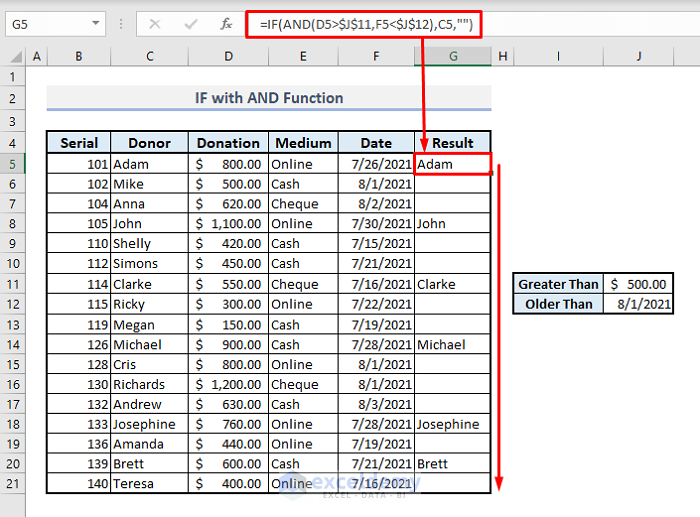
We’ll use a datasheet of donations, including the names, amounts, and dates. Let’s display the names of donors who have donated more than $500 before August 1, 2021. These two criterions will be listed in a separate table.
Steps:
- In the output Cell G5, insert this formula:
=IF(AND(D5>$J$11,F5<$J$12),C5,"")- Press Enter and autofill the entire column.
Let’s find out the names of the donors who have donated through cash or cheque from Column E.
Steps:
- In Cell G5, copy the following:
=IF(OR(E5=$J$11,E5=$J$12),C5,"")- Press Enter and autofill the entire column.

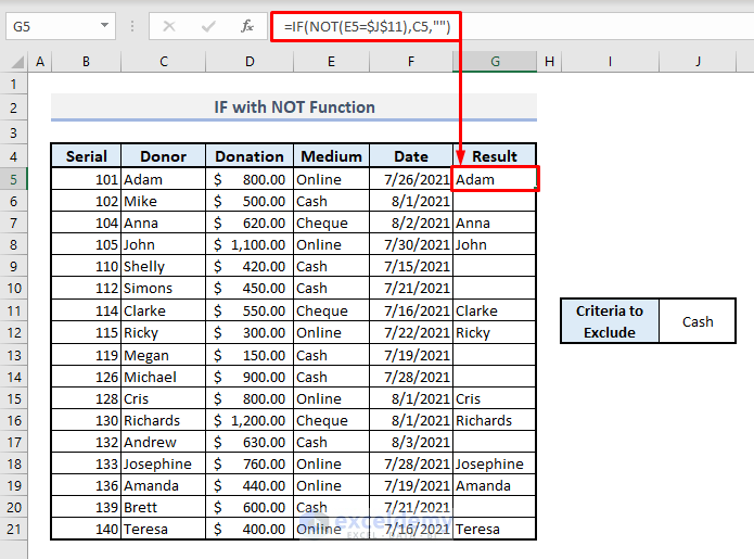
Let’s also list the donors who have not donated through cash, which is listed in a separate cell as an excluding criterion.
Steps:
- In Cell G5, copy the following:
=IF(NOT(E5=$J$11),C5,"")- Press Enter and auto-fill the rest of the cells.
Read More: How to Check If a Value Is Between Two Numbers in Excel
Method 5 – IF with ISBLANK, ISTEXT, ISNUMBER, and ISLOGICAL Functions
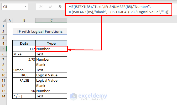
In the table below, we’ll find out in Column C what types of data are in the respective cells in Column B.
Steps:
- In the output Cell C5, copy the following formula:
=IF(ISTEXT(B5),"Text",IF(ISNUMBER(B5),"Number", IF(ISBLANK(B5),"Blank",IF(ISLOGICAL(B5),"Logical Value",""))))- Press Enter and autofill the entire column.
Read More: How to Use Multiple IF Statements with Text in Excel
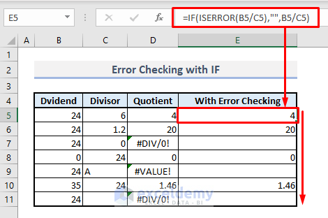
Method 6 – Error Checking by Combining IF and ISERROR Functions
Steps:
- Select the output Cell E5 and insert the following:
=IF(ISERROR(B5/C5),"",B5/C5)- Press Enter and autofill the entire column with the Fill Handle.
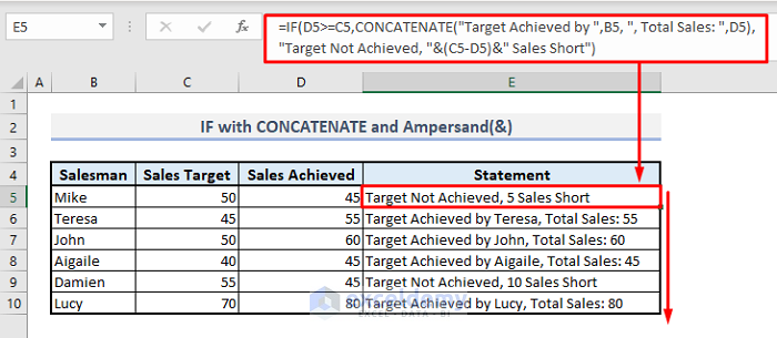
Method 4 – IF with Ampersand (&) or CONCATENATE Functions to Join Text and Numerical Values
Based on the sales dataset below, we’ll make some statements for those who have achieved the sales target and those who couldn’t
Steps:
- In Cell E5, copy the following formula:
=IF(D6>=C6,CONCATENATE("Target Achieved by ",B6, ", Total Sales: ",D6),"Target Not Achieved, "&(C6-D6)&" Sales Short")- Press Enter and autofill the entire column.
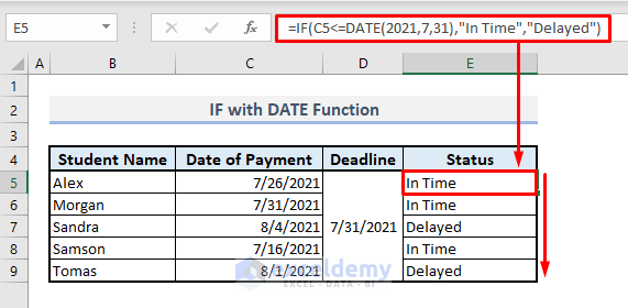
Method 8 – IF with DATE Function in Excel
Consider the deadline for the payment of tuition fees for July is 7/31/2021. We’ll find out the status of the students who paid the tuition fees in time and who couldn’t.
Steps:
- In the output Cell E5, the related formula will be:
=IF(C5<=DATE(2021,7,31),"In Time","Delayed")- Press Enter and fill down the entire column with the Fill Handle.
Read More: How to Use IF Formula with Dates
Things to Keep in Mind
In the arguments of IF function, although the 2nd argument [value_if_true] is considered optional, if you don’t input the statement there, the function will not be executed and a message will pop up to ask if you want to type a formula or make it a text value.
If you don’t define 2nd and 3rd arguments but just use a Comma(,), then the function will return 0 for any logical test.
The IF function can’t include more than one logic statement. You’ll need to use nested IF where multiple conditions can be added. Or, you can use the IFS function directly where you’ll find options to add multiple conditions.
If you want to sum based on a condition, then you can use directly SUMIF instead of combining IF and SUM functions. Similarly, to count cells based on conditions, it’s better to use COUNTIF in lieu of incorporating IF and COUNT functions.
Download Practice Workbook
You can download our Excel Workbook that we’ve used to prepare this article.
Excel IF Function: Knowledge Hub
<< Go Back to Excel Functions | Learn Excel
Get FREE Advanced Excel Exercises with Solutions!

