A number format is a standard way to present numerical values that can be easily understood by a wide audience. Different regions around the world use various number formats, each with its own conventions. Among these, the European and US number formats stand out. In this article, we’ll explore how to convert European number formats to the US format in Excel, complete with clear illustrations.
Difference Between European and US Number Formats
The primary distinction between European and US number formats lies in the use of decimal and thousand separators. Here’s how they differ:
- European Format:
- Decimal separator: Comma (,)
- Thousand separator: Decimal point (.)
- Example: 1.010,53
- US Format:
- Decimal separator: Decimal point (.)
- Thousand separator: Comma (,)
- Example: 1,010.53
Dataset Overview
We’ll work with a dataset of numbers in the European format and explore different techniques to convert them to the US format.
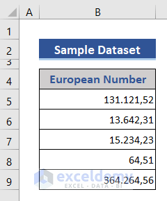
Method 1 – Using the NUMBERVALUE Function
- Add a new column to the right of your dataset.
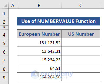
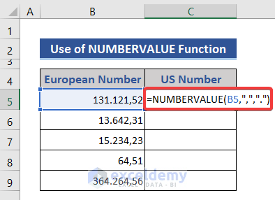
- In cell C5, enter the following formula:
=NUMBERVALUE(B5,",",".")
This formula converts the European number in cell B5 to a US-compatible numeric value.
- Press Enter and drag the Fill Handle icon to apply the formula to other cells.
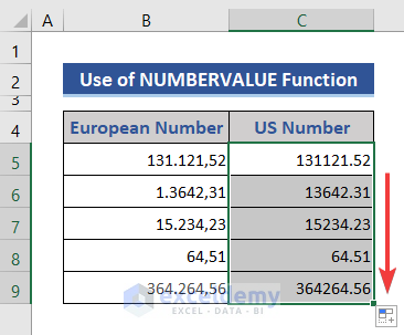
While the commas (,) are removed and decimal points added, there are no thousand separators yet.
To add thousand separators:
- Press Ctrl + 1 to open the Format Cells window.
- Choose the Number category from the Number tab.
- Tick the Use 1000 Separator (,) option.
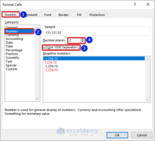
- Adjust the decimal places as needed.
- Click OK.
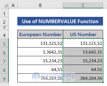
The numbers are now successfully converted to the US format.
Read More: How to Convert Percentage to Decimal in Excel
Method 2 – Using the SUBSTITUTE Function
- Insert the following formula in cell C5:
=SUBSTITUTE(SUBSTITUTE(B5, ".", "" ), ",", ".")+0
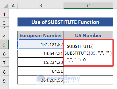
Formula Explanation:
- SUBSTITUTE(B5, “.”, “” )
Removes decimal points.
Result: 131121,52
- SUBSTITUTE(SUBSTITUTE(B5, “.”, “” ), “,”, “.”)
Replaces commas with decimal points.
Result: 131121.52
- SUBSTITUTE(SUBSTITUTE(B5, “.”, “” ), “,”, “.”)+0
Adding 0 converts the result from General to Number format.
Result: 131121.52
- Press Enter and drag the Fill Handle icon downward to apply the formula to other cells.
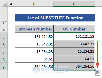
Note that we’ve already added commas as thousand separators (as shown in Method 1).
Read More: How to Convert Exponential Value to Exact Number in Excel
Method 3 – Using Excel’s Text to Columns Wizard to Convert Number Format from European to US
In this method, we’ll leverage the built-in Text to Columns feature in Excel to convert numbers from the European format to the US format.
Copying Data:
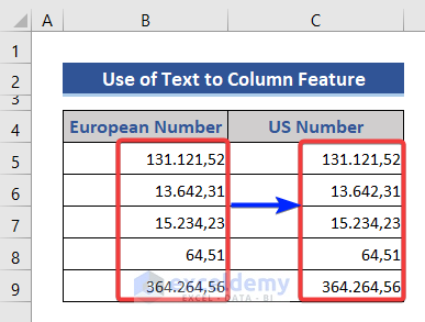
- Copy the numbers from the European Number column to the US Number column.
Accessing Text to Columns:
- Select the data in the US Number column.
- Go to the Data tab and click on Text to Columns.
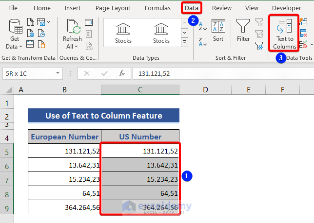
- The Convert Text to Columns Wizard window will appear.
Configuring Settings:
- Choose the Fixed Width option and click Next.
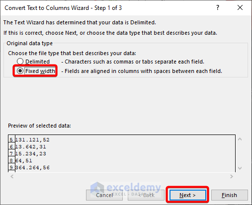
- Skip the second step of the wizard.
- Click Advanced in the third step.
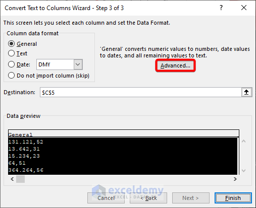
- In the Advanced Text Import Settings window:
- Set a comma (,) as the decimal separator.
- Set a decimal point (.) as the thousands separator.
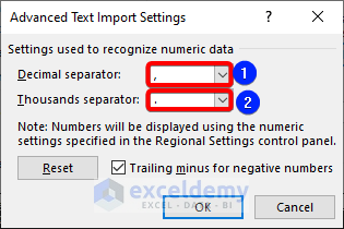
- Confirm the settings by pressing OK.
Finishing the Conversion:
- Click Finish in the Convert Text to Columns Wizard.
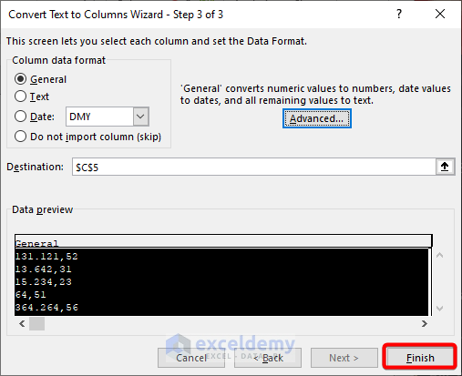
- Examine the dataset.
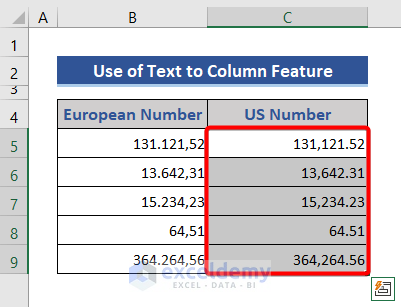
You’ll notice that the given numbers have been successfully converted into the US format.
Method 4 – Converting Number Formats Using VBA Macro
Now, let’s use a VBA (Visual Basic for Applications) macro to convert numbers from the European format to the US format. This VBA code works in two steps:
Accessing VBA Window:
- Go to the sheet name at the bottom of the Excel sheet.
- Right-click and choose View Code from the Context Menu.
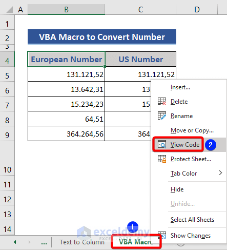
- The VBA window will appear.
Creating a Module and Adding Code:
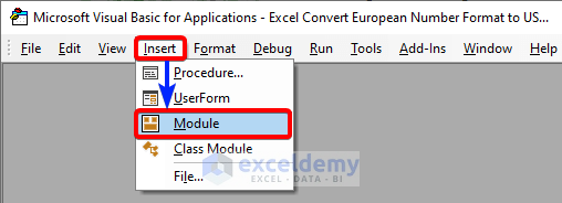
- Click on Insert and choose Module.
- Enter the following VBA code to the module window:
Sub Euro_to_US()
Selection.Replace What:=".", Replacement:="XXXXX", LookAt:=xlPart, _
    SearchOrder:=xlByRows, MatchCase:=False
Selection.Replace What:=",", Replacement:=".", LookAt:=xlPart, _
    SearchOrder:=xlByRows, MatchCase:=False
Selection.Replace What:="XXXXX", Replacement:=",", LookAt:=xlPart, _
    SearchOrder:=xlByRows, MatchCase:=False
End Sub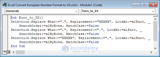
Running the VBA Code:
- Select a range of data.
- Press the F5 key to execute the VBA code.
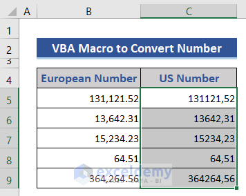
- The decimal points have been removed.
- Press F5 again to complete the conversion.
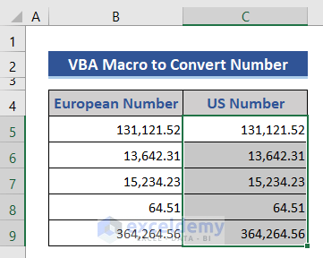
- The data is now in the US format.
Download Practice Workbook
You can download the practice workbook from here:
Related Articles
- [Solved] Excel Number Stored As Text
- Number Format Is Not Working in Excel
- [Solved!] Long Numbers Are Displayed Incorrectly in Excel
<< Go Back to Change Number Format | Number Format | Learn Excel


