To demonstrate the solutions, we’ll use a dataset of 10 employees of a company and their salaries. Our dataset is in the range of cells B5:C14.
Fix 1 – Avoid Non-Numeric Values
To display the dataset with the conditional formatting percentage format, we have to avoid the presence of non-numeric data in our dataset. You may notice that in the Income column, there is a non-numeric value. We cannot apply the conditional formatting data bar with percentages.
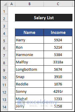
Steps:
- Select cell C8.
- Remove the non-numeric value from the cell.
- Press Enter.
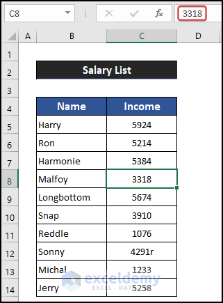
- Remove the non-numeric value from cell C12.
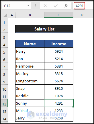
- Apply the conditional formatting data bar with percentage formatting, and you will get the result.
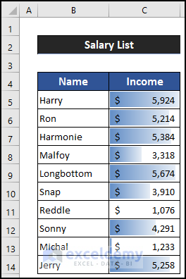
Fix 2 – Choosing Percent Formatting
Steps:
- Select the range of cells C5:C14.
- Click on the drop-down arrow of the Conditional Formatting, then choose the Data Bars option and select the More Rules option.
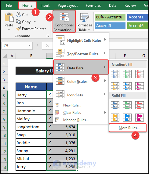
- A small dialog box called New Formatting Rules will appear.
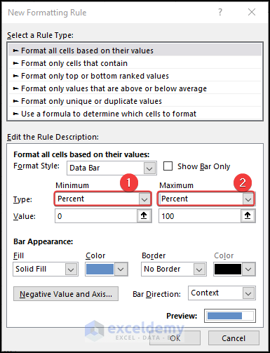
- In the Type option, click on the drop-down arrow of the Minimum option and change the option from Automatic to Percent.
- Change the Type option for the Maximum value from Automatic to Percent.
- The Minimum and the Maximum values will be automatically set by Excel. The Minimum value of 0 will be the lowest value of the dataset, and the Maximum value of 100 will be the highest value of the dataset.
- Select the Fill type. We choose the Gradient Fill option.
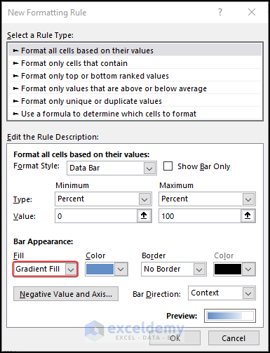
- Click on OK.
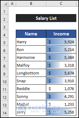
Read More: How to Use Data Bars with Percentage in Excel
Fix 3 – Applying Automatic Formatting
Steps:
- Select the range of cells C5:C14.
- In the Home tab, click on the drop-down arrow of the Conditional Formatting, then go to the Data Bars option and choose the More Rules option.

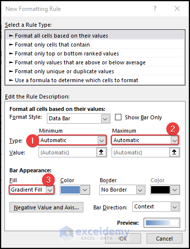
- A small dialog box called New Formatting Rules will appear.
- Keep the Type option for both Minimum and Maximum as Automatic.
- Click on the drop-down arrow of the Fill option and choose an option. We choose Gradient Fill.
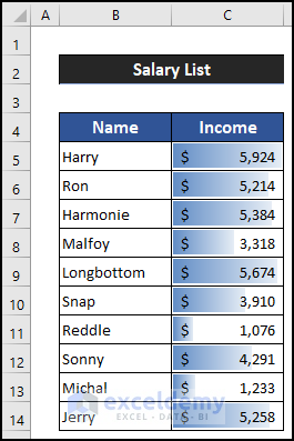
- Click on OK.
Fix 4 – Show Data Bars Separately
Steps:
- Select the range of cells C5:C14 and press Ctrl + C to copy the data.
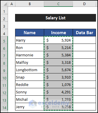
- Select cell D5 and press Ctrl + V to paste the data.
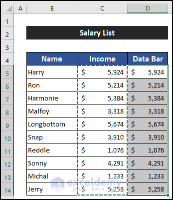
- Select the range of cell D5:D14.
- In the Home tab, click on the drop-down arrow of the Conditional Formatting, then go to the Data Bars option and choose the More Rules option.
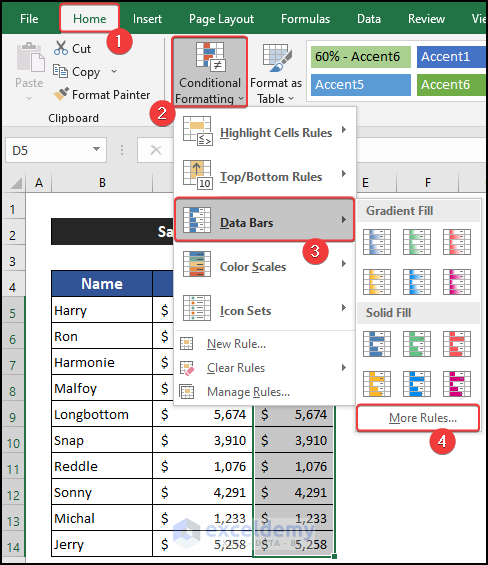
- A small dialog box called New Formatting Rules will appear.
- In the Type option, click on the drop-down arrow of the Minimum option and change the option from Automatic to Percent.
- Change the Type option for the Maximum value from Automatic to Percent.
- Excel will automatically set the Minimum and the Maximum values. Here, the Minimum value of 0 will be the lowest value of the dataset, and the Maximum value of 100 will be the highest value of the dataset.

- Select the Fill type. We choose the Gradient Fill option.

- Check the Show Bar Only option.
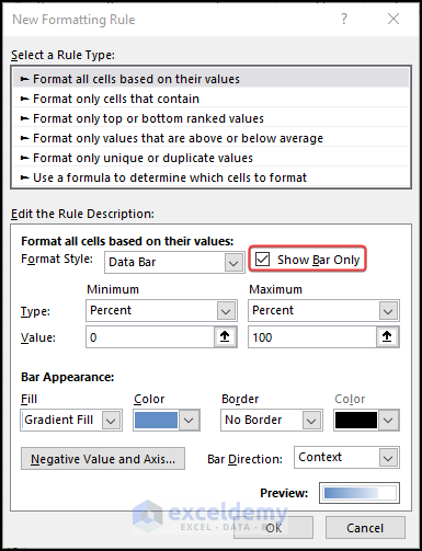
- Click OK.
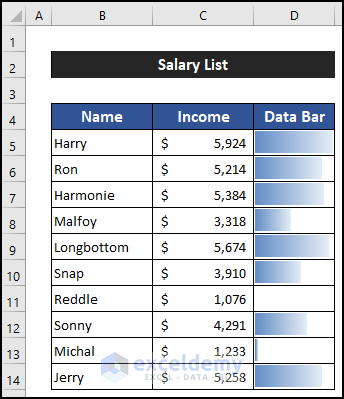
Fix 5 – Re-Installing an Updated Version of Excel
An updated version of Excel neglects the cell format of the Number group, and it automatically sets the cell formatting by the cell entities.
Download the Practice Workbook
Related Articles
- How to Add Data Bars in Excel
- How to Add Solid Fill Data Bars in Excel
- How to Define Maximum Data Bars Value in Excel
- Conditional Formatting with Data Bars Based on Another Cell in Excel
- Conditional Formatting Data Bars Different Colors
<< Go Back to Data Bars | Conditional Formatting | Learn Excel
Get FREE Advanced Excel Exercises with Solutions!

