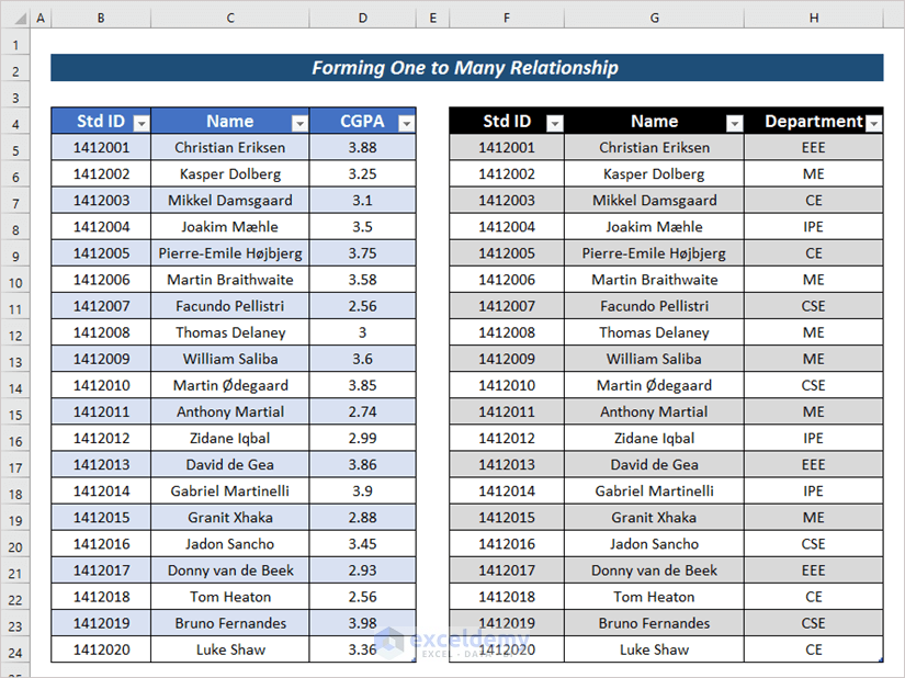
Method 1 – Make a One-to-Many Relationship with a Formula
Steps:
- Organize two co-related datasets.
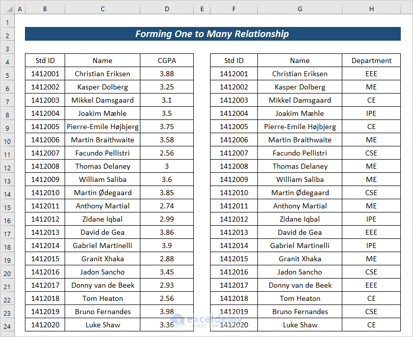
- Form tables with both datasets.
- Select the entire first dataset.
- Go to the Insert tab and click on Table from the ribbon.
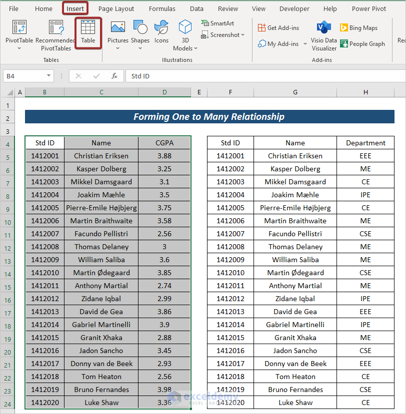
- Set your table range and press OK.

Table1 will be created.
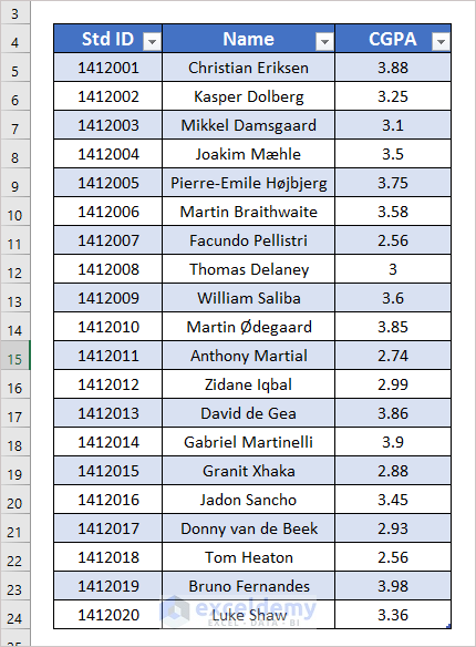
- Use the same procedure to make Table2 from the second dataset.
- Select a cell (i.e. K5) and input the following formula to get the average CGPA of all the departments.
=AVERAGE(IF(COUNTIFS(Table2[Std ID],Table1[Std ID],Table2[Department],J5),Table1[CGPA]))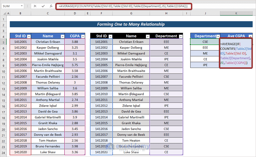
- Press Enter.
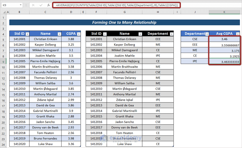
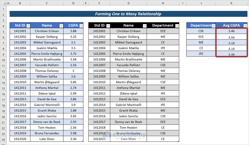
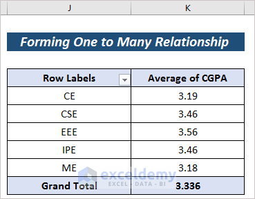
We can further modify the output to format it.
Read More: How to Create Many to Many Relationship in Excel
Method 2 – Make a One-to-Many Relationship with a PivotTable
Steps:
- Put the dataset into tables.
- Go to the Power Pivot tab.
- Click on Manage from the ribbon.
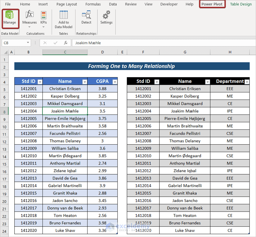
Power Pivot for Excel will appear.
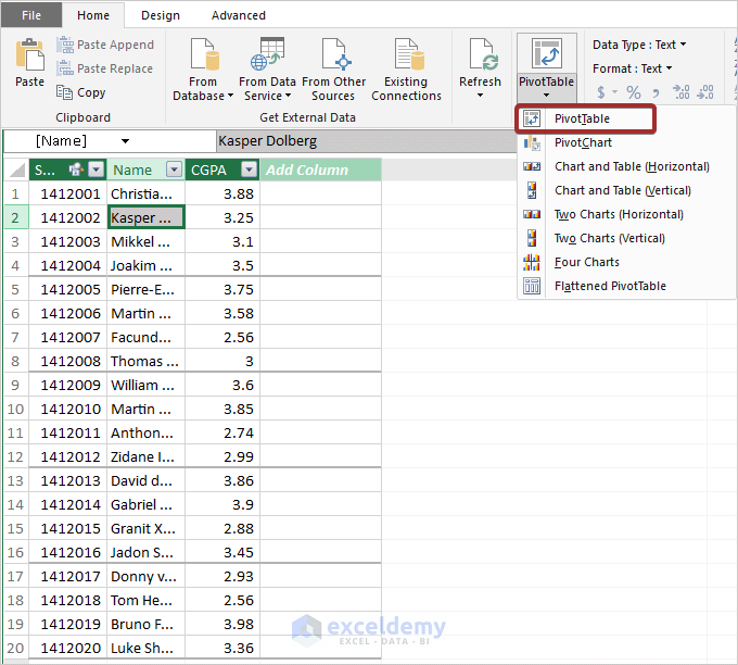
- Go to PivotTable from the ribbon under the File tab.
- Select PivotTable.
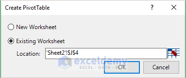
- Pick your PivotTable location and click on OK.
- From the PivotTable Fields, manage your PivotTable. We have set Department as Rows and Sum of CGPA as values.
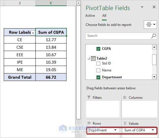
We will get the sum of CGPA for all the departments.
- Right-click on the Sum of CGPA title.
- Pick Average from the Summarize Values By group.
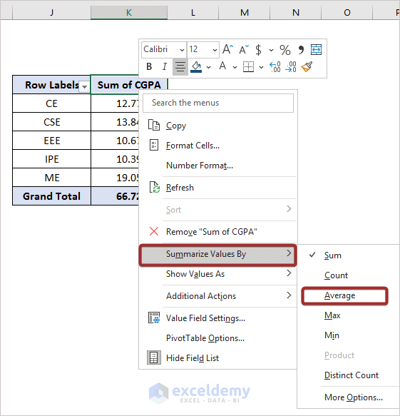
We will get the average CGPA for all the departments.
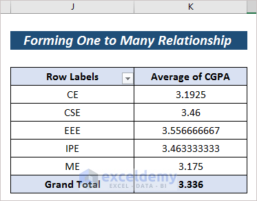
You can modify your output based on your preferences.
Practice Section
For further expertise, you can practice with the download file.
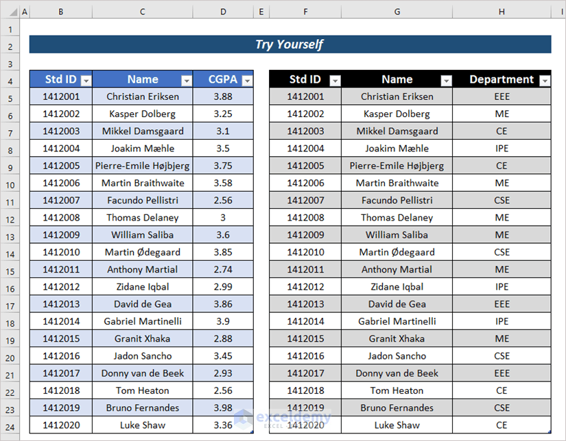
Download the Practice Workbook
Related Articles
- How to Create Data Model Relationships in Excel
- How to Create Relationship in Excel with Duplicate Values
- Create Entity Relationship Diagram from Excel
- How to Manage Relationships in Excel
- How to Create Table from Data Model in Excel
- [Fixed!] Excel Data Model Relationships Not Working
<< Go Back to Create Relationships in Excel | Data Model in Excel | Learn Excel
Get FREE Advanced Excel Exercises with Solutions!
