Method 1 – Merging Multiple Columns to Create Table from Another Table in Excel
Steps:
- We use the table below for this example:
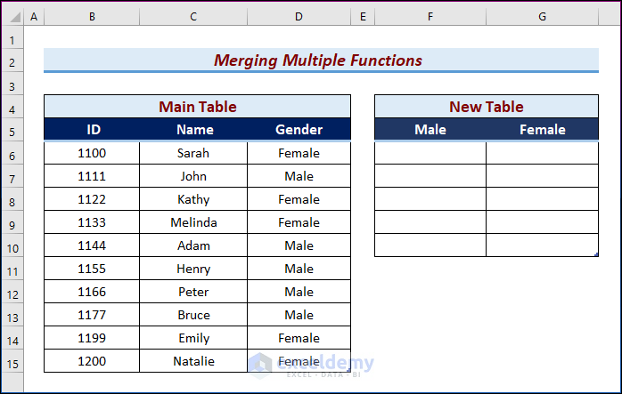
- Select cell F6.
- Enter the following formula:
=IFERROR(INDEX($C$6:$C$15,SMALL(IF($D$6:$D$15=F$5,(ROW($D$6:$D$15)-5),FALSE),ROW()-5)),"")- Press Enter.
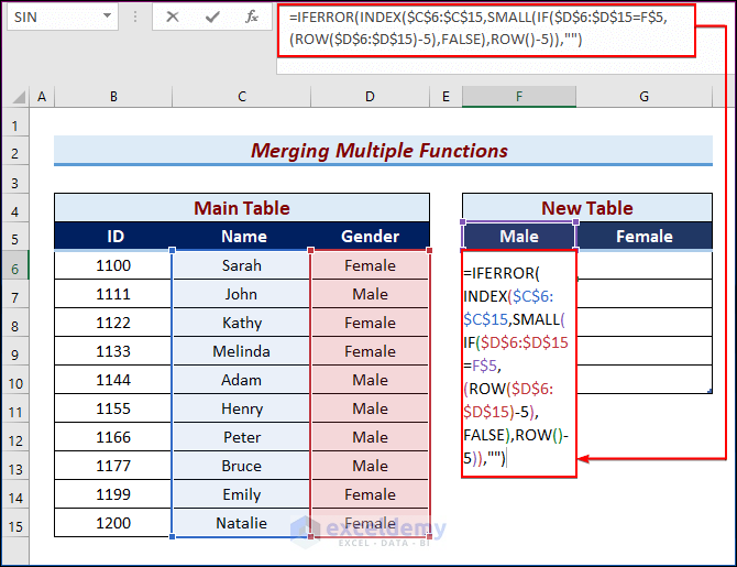
- ROW($D$6:$D$15)-5),FALSE),ROW()-5): The ROW function returns the row number for reference.
- IF($D$6:$D$15=F$5,(ROW($D$6:$D$15)-5),FALSE): This section returns the value after checking the condition whether it is true or false.
- SMALL(IF($D$6:$D$15=F$5,(ROW($D$6:$D$15)-5),FALSE),ROW()-5)),””): The SMALL function outputs a numeric number based on its position inside a list when the values are sorted in ascending order.
- INDEX($C$6:$C$15,SMALL(IF($D$6:$D$15=F$5,(ROW($D$6:$D$15)-5),FALSE),ROW()-5)),””): The INDEX function extracts a value from a table or range, or a reference to a value, and returns it.
- =IFERROR(INDEX($C$6:$C$15,SMALL(IF($D$6:$D$15=F$5,(ROW($D$6:$D$15)-5),FALSE),ROW()-5)),””): The IFERROR function represents the correct result if there is an error.
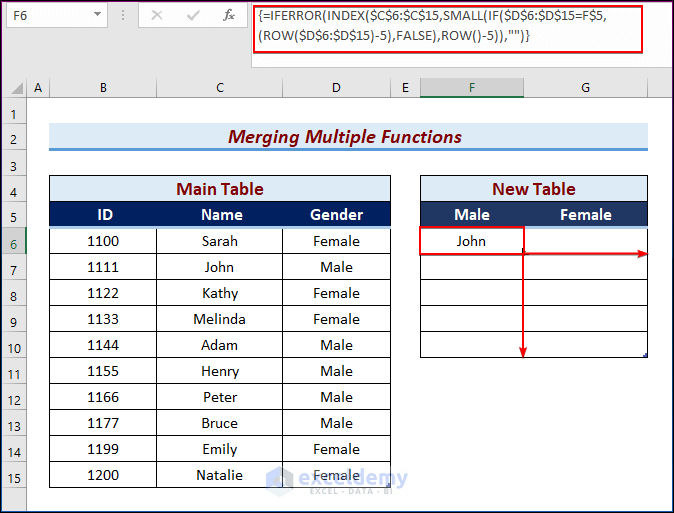
- You will now see the first employee’s name in the New Table.
- Use the Fill Handle tool and drag it to see all the employee names.
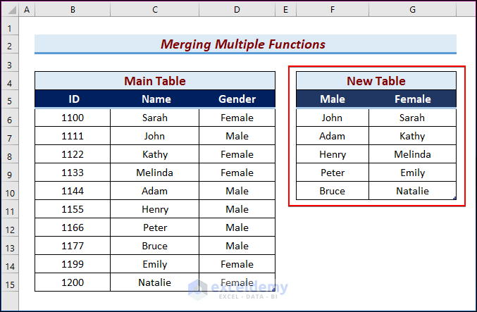
- You will have the following result.
Read More: How to Create Table from Multiple Sheets in Excel
Method 2 – Combining VLOOKUP and COLUMN Functions to Create Table from Another Table in Excel
Let’s say you have two tables and a dataset of employees. Sample Table 1 has the Employee Name and ID columns. Sample Table 2 has two columns with the names Joining Date and ID. Here’s what to do if you want to add the joining dates from Sample Table 2 to your New Table.
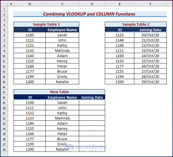
Steps:
- Select cell D19.
- Enter the following formula.
=IFERROR(VLOOKUP($B19,$E$6:$F$15,COLUMN(B18),FALSE),"")- Hit Enter.
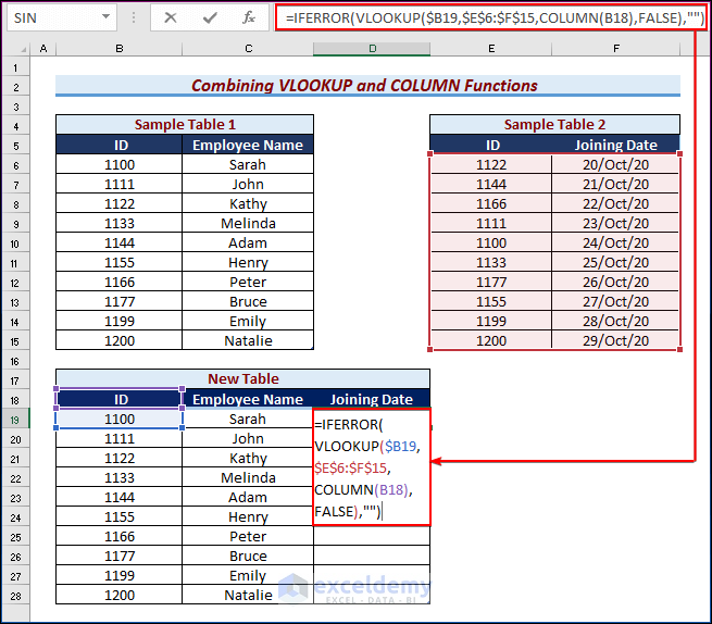
- COLUMN(B18): The COLUMN function returns the particular column number.
- VLOOKUP($B19,$E$6:$F$15,COLUMN(B18): This portion shows a certain value for a specified range.
- =IFERROR(VLOOKUP($B19,$E$6:$F$15,COLUMN(B18),FALSE),””): The IFERROR function represents the correct result if there is any error.
- You will now see the first employee’s joining date.
- Now use the Fill Handle tool and drag it down from the D19 cell to the D28 cell.
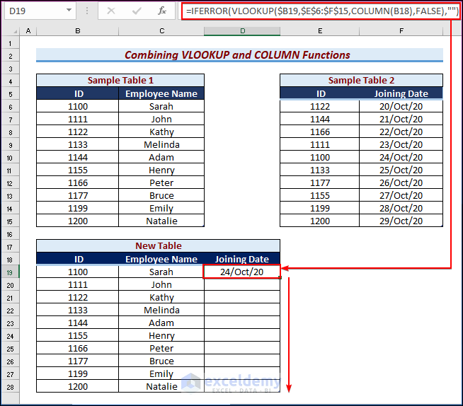
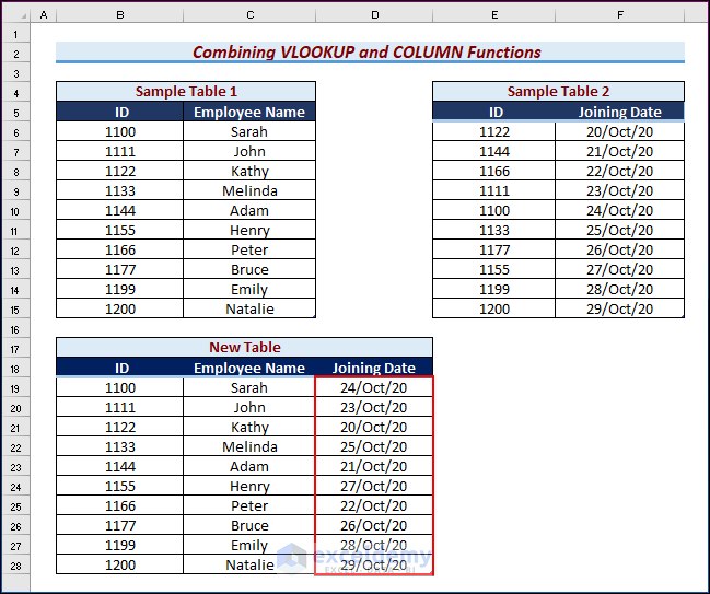
- You will now get all the employees joining dates as shown in the below image.
Read More: How to Mirror Table on Another Sheet in Excel
Method 3 – Nesting INDEX and MATCH Functions to Create Table from Another Table in Excel
In this example we have two tables, Sample Table 1 and Sample Table 2. Imagine you have to add the employee’s IDs to Sample Table 2.
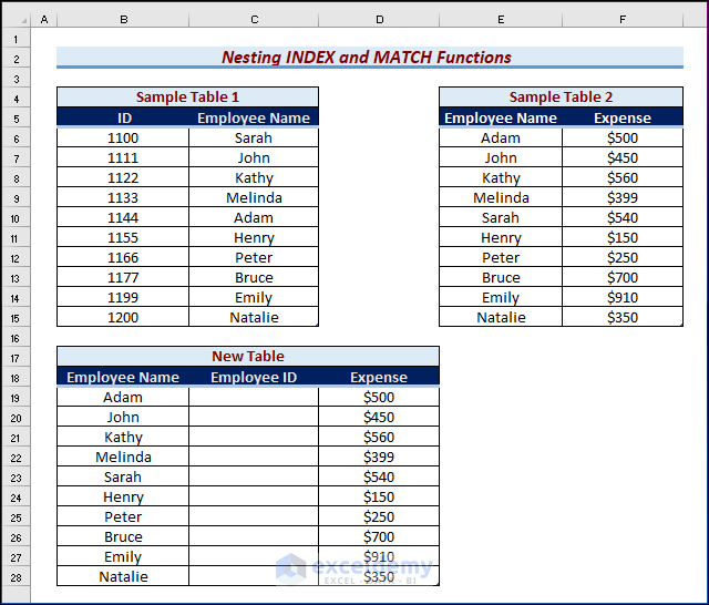
Steps:
- Select cell C19..
- Enter the following formula.
=INDEX(Sample_Table1,MATCH(B19,Sample_Table1[Employee Name],0),1)
- Hit Enter.
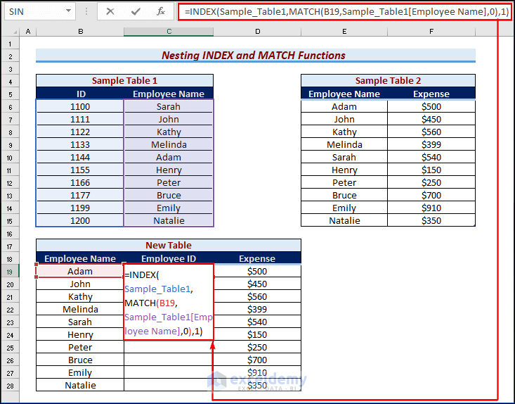
- MATCH(B19,Sample_Table1[Employee Name],0): The MATCH function looks for a specific item within a set of cells, finds it, and then returns the item’s position within the set of cells.
- =INDEX(Sample_Table1,MATCH(B19,Sample_Table1[Employee Name],0),1): This INDEX function extracts a value from a table or range, or a reference to a value, and returns it.
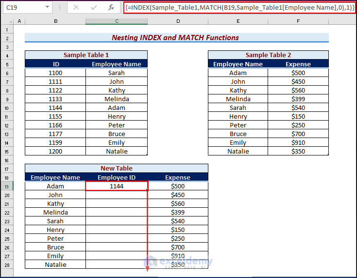
- You will now see the first employee’s ID in the below image.
- Now use the Fill Handle tool and drag it down from cell C19 to cell C28.
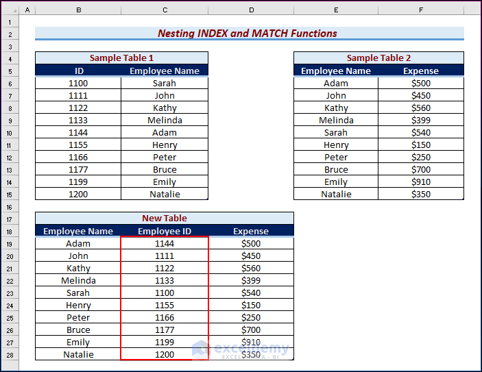
- You will now see all employee IDs listed.
Read More: How to Create Table from Another Table with Criteria in Excel
Download Practice Workbook
You may download the following Excel workbook for better understanding and practice it yourself.
Related Articles
- How to Create a Lookup Table in Excel
- How to Make 3D Table in Excel
- How to Make a Decision Table in Excel
- How to Create a League Table in Excel
- How to Make a Table Bigger in Excel
<< Go Back to Excel Table | Learn Excel
Get FREE Advanced Excel Exercises with Solutions!

