This is an overview of the SEARCH function.
Introduction to the SEARCH Function
- Summary
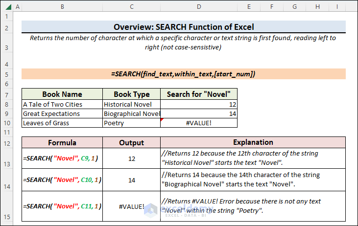
The SEARCH function returns the number of characters after finding a specific character or text string, reading from the left to the right. This function searches for a case-insensitive match. It works for both Array and Non-Array Formulas.
- Syntax
The syntax of the SEARCH function is:
SEARCH(find_text,within_text,[start_num])
- Arguments
| ARGUMENT | REQUIREMENT | EXPLANATION |
|---|---|---|
| find_text | Required | The text that is searched can be a single text or an array. |
| within_text | Required | The text value within which the find_text argument is searched for can be a single text value or an array of text values. |
| [start_num] | Optional | The position of the within_text argument from which it starts searching can be a single number or an array of numbers. Default is 1. |
Note:
- If at least one of the arguments is an array, the formula will turn into an Array Formula and you need to press Ctrl + Shift + Enter to enter the formula.
Example 1- Filtering the First Names
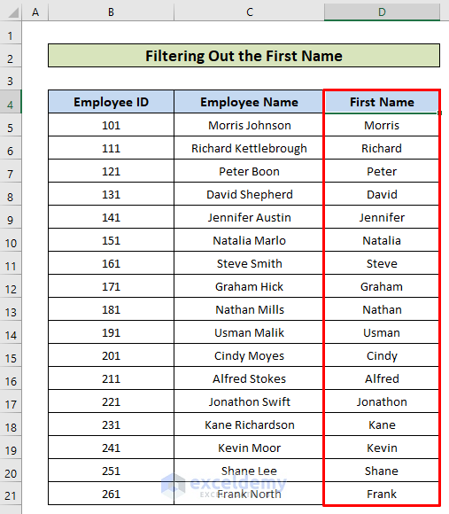
The dataset below showcases Employee IDs and Employee Names.
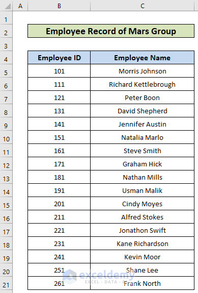
To extract the first names:
Steps:
- In D5, enter this formula:
=LEFT(C4,SEARCH(" ",C4,1)-1)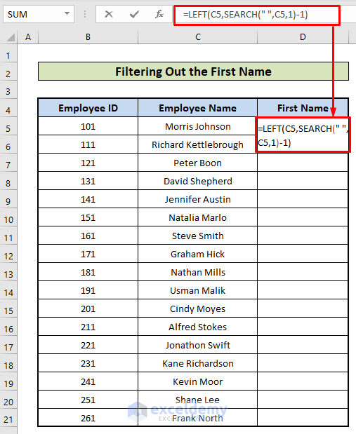
- Press Enter.
- The first name of the first employee is displayed. Drag down the Fill Handle to apply the formula to the rest of the cells.
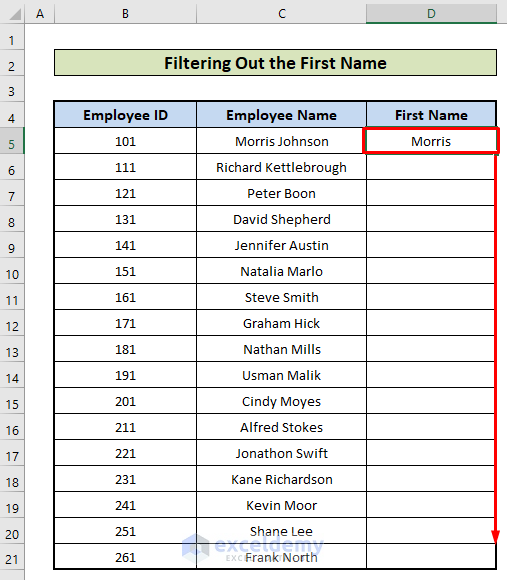
This is the output.
Formula Breakdown
- SEARCH(” “,C4,1): shows where there is a space (“ “) in the name within C4.
- LEFT(C4,SEARCH(” “,C4,1)-1): Extracts the string before the space from the left.
See the LEFT function for details.
Example 2 – Filtering a Specific Type of Book from a List of Books
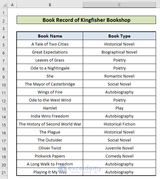
The dataset showcases books titles and their types.
Steps:
- Enter this formula in the first cell of a new column:
=IF(ISNUMBER(SEARCH("Novel",C4,1)),"Yes","No")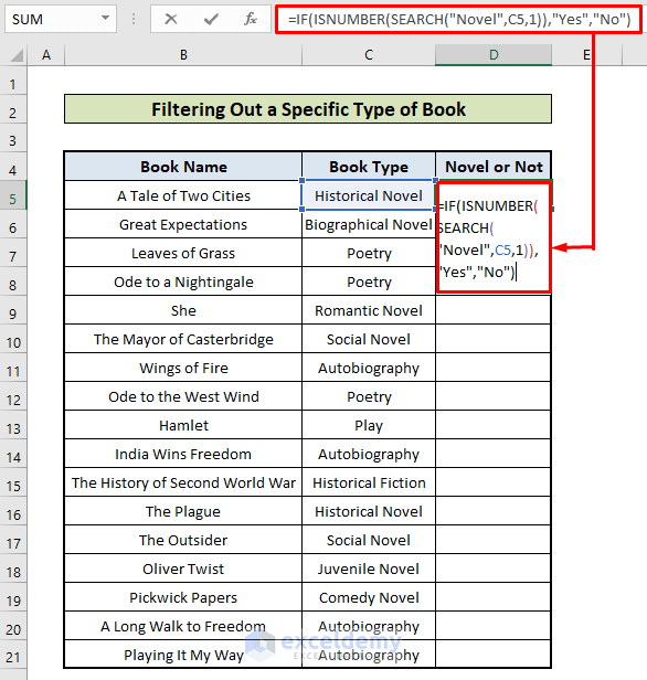
- Double-click the Fill Handle to fill the rest of the cells.
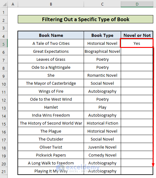
This is the output.
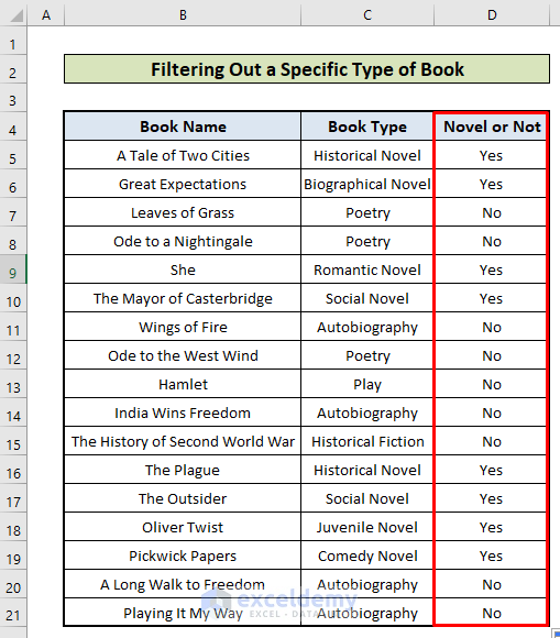
Formula Breakdown
- SEARCH(“Novel”,C4,1): Searches “Novel” in the book type column. If it finds a match, it returns a number. Otherwise, #VALUE! Error.
- ISNUMBER(SEARCH(“Novel”,C4,1)): Converts the number into TRUE, and the error into FALSE.
- IF(ISNUMBER(SEARCH(“Novel”,C4,1)),”Yes”,”No”): Returns “Yes” if it finds TRUE, and “No” if it finds FALSE.
Example 3 – Using an Array Formula with the SEARCH Function
Consider the dataset in Example 1. To extract the first names from all names:
Steps:
- Apply an Array Formula. The formula is:
=LEFT(C4:C20,SEARCH(" ",C4:C20,1)-1)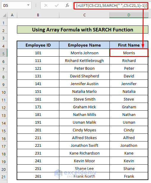
It returns the first names from all names simultaneously.
Formula Breakdown
The formula LEFT(C4:C20,SEARCH(” “,C4:C20,1)-1) consists of 17 single formulas.
- LEFT(C4,SEARCH(” “,C4,1)-1)
- LEFT(C5,SEARCH(” “,C5,1)-1)
- LEFT(C6,SEARCH(” “,C6,1)-1)
…
…
…
- LEFT(C20,SEARCH(” “,C20,1)-1)
Each of them extracts the first name from the full names (See Example 1). The formula searches for a space(“ ”) in each cell in C4:C20 and extracts the strings before the space in all cells, starting from the left.
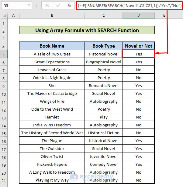
Consider the dataset in Example 2. Use the Array Formula.
Steps:
- Copy the following formula.
=IF(ISNUMBER(SEARCH("Novel",C4:C20,1)),"Yes","No")- Press enter to see the result.
Download Practice Workbook
<< Go Back to Excel Functions | Learn Excel
Get FREE Advanced Excel Exercises with Solutions!

