In this article, we will demonstrate some uses of the SUBSTITUTE function with examples.
Excel SUBSTITUTE Function: Quick View
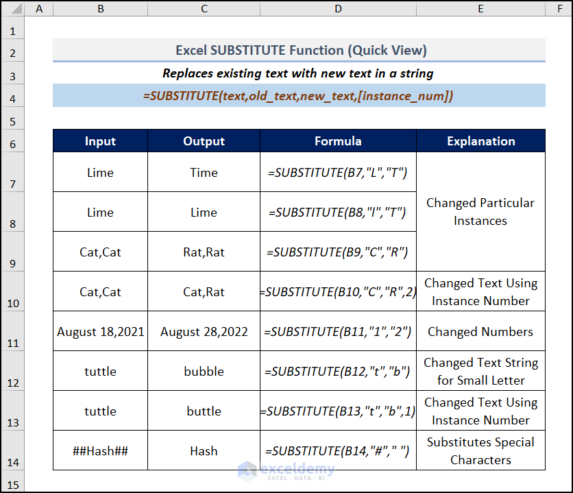
Introduction to the SUBSTITUTE Function in Excel
The SUBSTITUTE function is categorized under the Text functions category in Excel’s function library. It replaces matching text in a given string.
Summary:
Replaces existing text with new text in a text string.
Syntax:
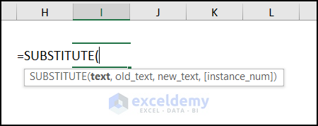
=SUBSTITUTE(text, old_text, new_text, [instance_num])
Argument Explanation:
| Argument | Required/Optional | Explanation |
|---|---|---|
|
text |
Required |
The text to change |
|
old_text |
Required |
The text to be replaced |
|
new_text |
Required |
The text with which to replace old_text |
|
instance_num |
Optional |
The instance of old_text to replace in text. |
Versions:
Available from Excel 2007 onwards.
How to Use the SUBSTITUTE Function in Excel: 7 Examples
Now we’ll present some basic examples of the SUBSTITUTE function. We’ll also demonstrate the difference between the SUBSTITUTE and REPLACE functions.
Example 1 – Making Changes to the Original String
Consider the following dataset consisting of a few random text strings.
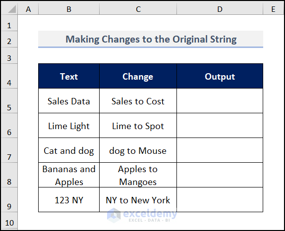
Let’s change some of the text using the SUBSTITUTE function.
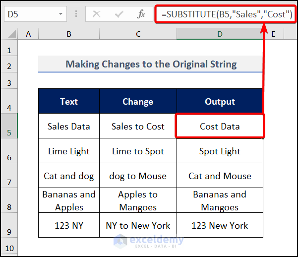
- Enter the following formula in cell D5 and press ENTER..
=SUBSTITUTE(B5,"Sales","Cost")Here, B5 is the text, our target word is “Sales”, and the word will be changed to “Cost”.
After applying the same process to the rest of column D, the result is as follows:
Example 2 – Changing a Particular Instance
Suppose the text we want to replace occurs multiple times within the text. We can change a particular instance by providing the instance number as the last argument in the SUBSTITUTE function.
In our sample dataset, every row contains redundant letters. Suppose we want to replace the lower case starting s in superstar in cell B5 with an upper case S.
- Enter the following formula in cell C5:
=SUBSTITUTE(B5, "s", "S")This function changes all the “s” characters to “S”.
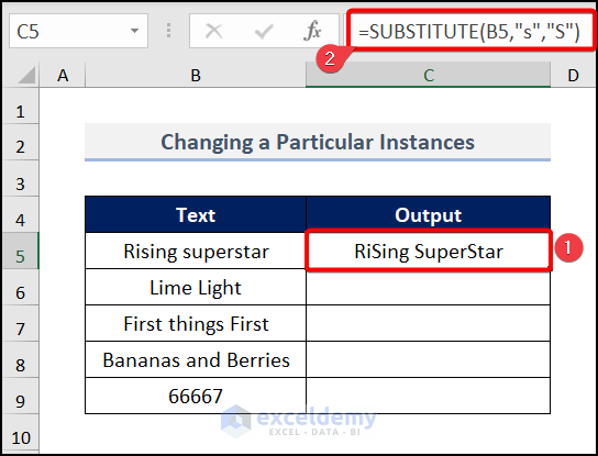
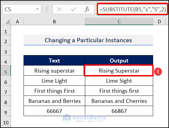
But we only wanted the first lowercase “s” changed, not all three, so we need to specify the instance number. Here, we want to change the string’s second “s“, so we enter 2 for the instance_num argument.
- Enter the following modified formula in cell C5:
=SUBSTITUTE(B5, "s", "S",2)Now, only the correct instance of “s” has been replaced by “S”.
Example 3 – Changing a Special Character
Suppose we need to replace a special character with another character. In the dataset below, let’s replace the (–) sign with the (*) sign using the SUBSTITUTE function.
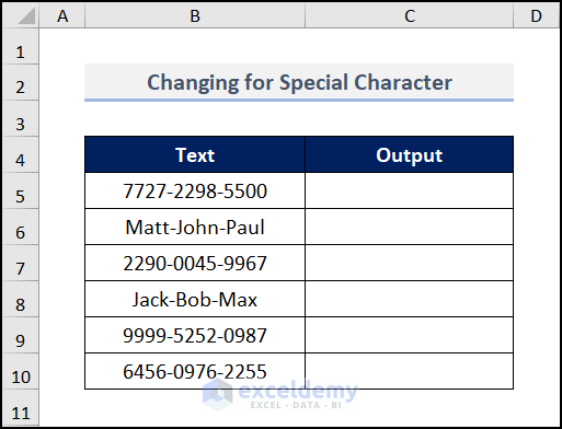
- In cell C5 insert the following formula:
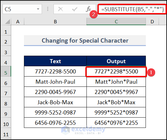
=SUBSTITUTE(B5,"-","*")The SUBSTITUTE(B5,”-“,”*”) syntax replaces all the (–) signs with the (*) sign.
The outcome is as in the image below.
Method 4 – Nested SUBSTITUTE Functions for Multiple Changes
A single SUBSTITUTE function will change one text at a time. To change multiple strings at once, we’ll need to use multiple SUBSTITUTE functions together.
Consider the following dataset of a few footballers with their abbreviated names and numbers.
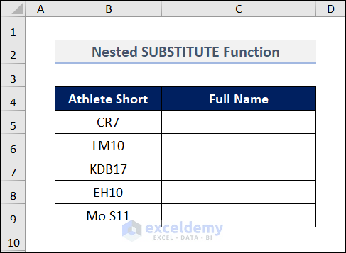
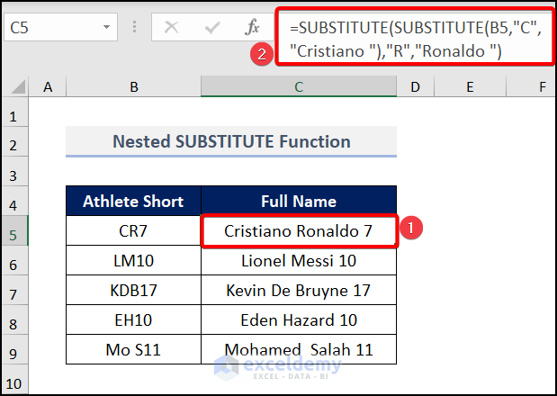
Let’s find the full name from the short name. The short name consists of the first and last name initials. We’ll replace the initials with the unabbreviated names using nested SUBSTITUTE functions.
- In cell C5 enter the following formula:
=SUBSTITUTE(SUBSTITUTE(B5,"C","Cristiano "),"R","Ronaldo ")The inner SUBSTITUTE function operates first, changing CR7 to Cristiano R7. The output is passed to the outer SUBSTITUTE function, which replaces R with Ronaldo to produce the final output.
Example 5 – Word Count Using the SUBSTITUTE Function
We can count the number of words present in a string using the SUBSTITUTE function, in conjunction with the LEN and TRIM functions.
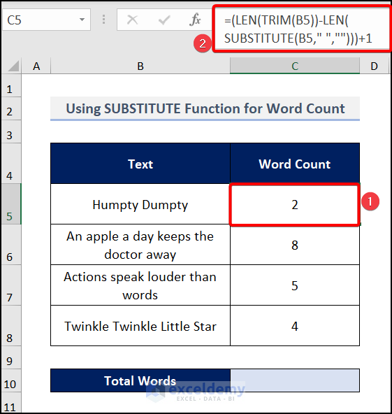
- In cell C5 enter the following formula:
=(LEN(TRIM(B5))-LEN(SUBSTITUTE(B5," ","")))+1Formula Explanation:
The SUBSTITUTE function removes all spaces from the string, and then LEN calculates the length without spaces.
This number is then subtracted from the length of the text with spaces. We use the TRIM function to remove any spaces at the beginning or end of the string.
Finally, 1 is added to the result, since the number of words is the number of spaces + 1.
- Press ENTER and drag the formula down to the cells below using the Fill Handle.
To find the total number of words in the range, we can use the SUMPRODUCT function with the previous formula.
- The formula is follows:
=SUMPRODUCT(LEN(TRIM(B5:B8))-LEN(SUBSTITUTE(B5:B8," ",""))+1)The function works like previously, but this time we have provided a range, so the inside portion of the SUMPRODUCT function returns an array of word counts for every row.
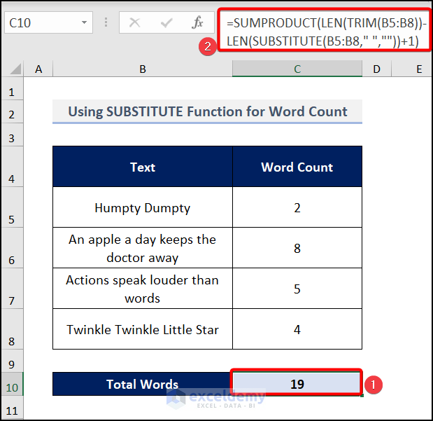
The total word count is returned, as shown in the above image.
Example 6 – Retrieve a Specified String Based on the Delimiter
Consider the following dataset of Products with their Product Ids. Let’s retrieve the last part of the Product Id based on the delimiter (“-“).
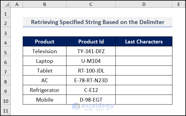
- In cell D5 enter the following formula:
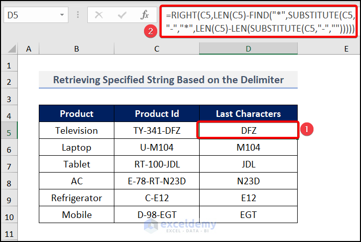
=RIGHT(C5,LEN(C5)-FIND("*",SUBSTITUTE(C5,"-","*",LEN(C5)-LEN(SUBSTITUTE(C5,"-","")))))Formula Explanation:
SUBSTITUTE(C5,”-“,””)→ Substitutes the (-) sign with nothing in cell C5.
- Output → TY341DFZ
LEN(SUBSTITUTE(C5,”-“,””)→ Counts the length of the string.
- Output → 8
LEN(C5)-LEN(SUBSTITUTE(C5,”-“,””)→ Subtracts the total length of the string with “-” characters removed from the original string length.
- Output → 10 – 8 = 2
SUBSTITUTE(C5,”-“,”*”,LEN(C5)-LEN(SUBSTITUTE(C5,”-“,””)→ Converts the (-) to the (*). However, it substitutes one (–) for the last instance.
FIND(“*”,SUBSTITUTE(C5,”-“,”*”,LEN(C5)-LEN(SUBSTITUTE(C5,”-“,””))→ Searches for the text before the (*) sign.
- Output → 7
LEN(C5)-FIND(“*”,SUBSTITUTE(C5,”-“,”*”,LEN(C5)-LEN(SUBSTITUTE(C5,”-“,””)))→ Subtracts the result from the total length of the string from the result of the FIND function.
- Output → 10 – 7 = 3
RIGHT(C5,LEN(C5)-FIND(“*”,SUBSTITUTE(C5,”-“,”*”,LEN(C5)-LEN(SUBSTITUTE(C5,”-“,””)))))→ The RIGHT function takes the output value of these functions and returns the text value.
- Output → DFZ
- Press ENTER and drag the same formula down to the rest of the cells in the column.
The result is as in the image below.
Example 7 – Using the SUBSTITUTE Function for Multiple Characters
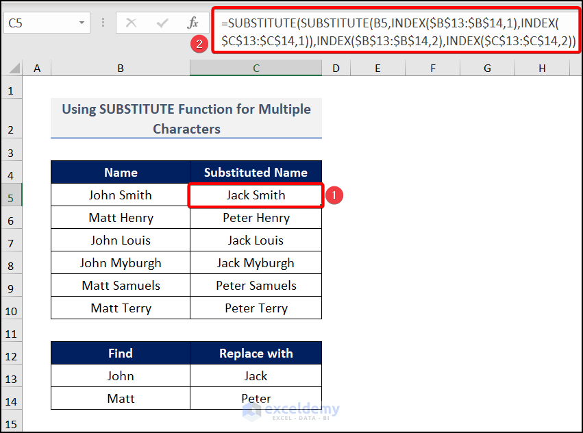
We can change multiple strings using the SUBSTITUTE and INDEX functions together. The INDEX function finds the value to change, and the SUBSTITUTE function then changes it.
- In cell C5 enter the following formula:
=SUBSTITUTE(SUBSTITUTE(B5, INDEX($B$13:$B$14,1), INDEX($C$13:$C$14,1)), INDEX($B$13:$B$14,2), INDEX($C$13:$C$14,2))Here, $B$13:$B$14 is the text we want to change, and $C$13:$C$14 is the text we want after changing.
- Press ENTER and drag down the Fill Handle to return the output below.
SUBSTITUTE vs REPLACE Function in Excel: What’s the Difference?
- The SUBSTITUTE function is a simpler but more comprehensive alternative to the REPLACE function. The REPLACE function is only suitable when the numerical start_num and num_chars arguments are known. The SUBSTITUTE function on the other hand, doesn’t require the start_num or num_char arguments. It only requires the cell name, the word or the text to be substituted, and the substitute word.
Common Errors While Using the SUBSTITUTE Function
| Error | Cause of Error | Solution |
|---|---|---|
|
#NAME? |
The function name is spelled incorrectly. |
Enter the function name correctly. |
Download Practice Workbook
<< Go Back to Excel Functions | Learn Excel
Get FREE Advanced Excel Exercises with Solutions!

