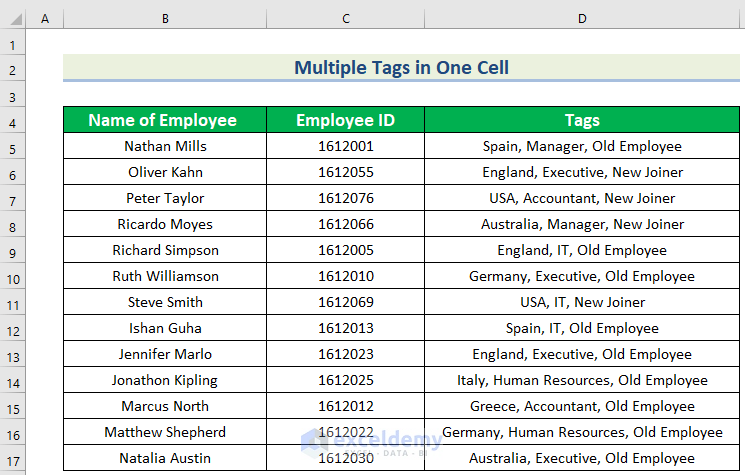
The following dataset contains three columns: Employee’s Name, ID, and Tags. The Tags column contains three types of information.
To find managers only:
Method 1 – Use Text Filters for Multiple Tags in One Cell
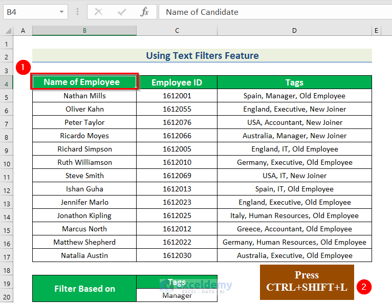
- Select any cell and press CTRL+SHIFT+L.
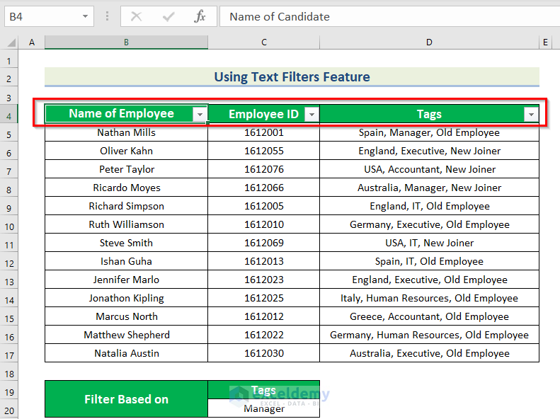
You will see a drop-down arrow beside every column header.
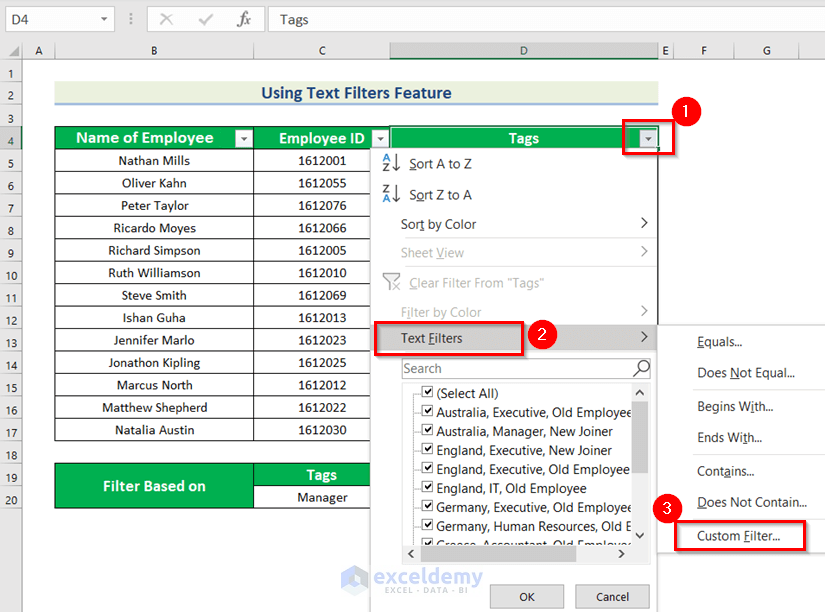
- Click the drop-down arrow in “Tags”.
- Go to Text Filters.
- Choose Custom Filter.
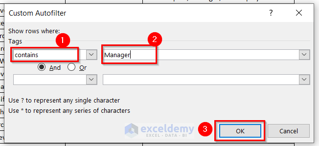
The Custom Autofilter dialog box will be displayed.
- Choose contains in the 1st drop-down arrow.
- Enter Manager in the second space.
- Click OK.
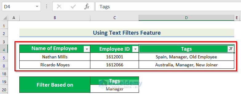
This is the output.
Read More: How to Add Tags in Excel
Method 2 – Applying an Advanced Filter in Excel
To find the “Employee Name” of managers:
Steps:
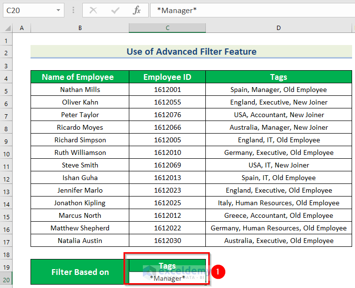
- Enter the criteria including Asterisks:
Tags >> *Manager* in C19:C20.
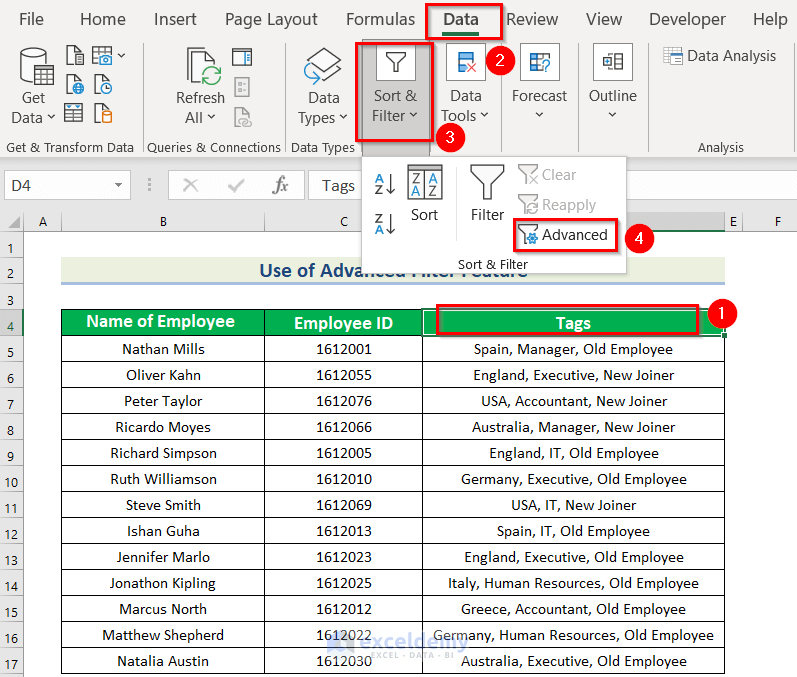
- Select any cell in the dataset.
- Open the Advanced Filter by clicking the Data tab > Sort & Filter > Advanced.
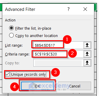
In Advanced Filter:
- Specify the range of your whole dataset in List range.
- Enter the criteria in Criteria range.
- Check Unique records only.
- Click OK.
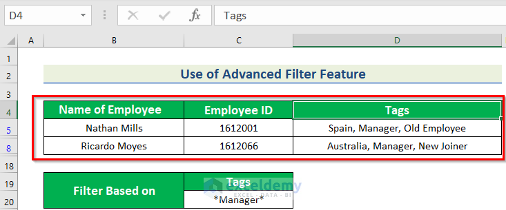
This is the output.
Read More: How to Add Tag to Properties in Excel
Method 3 – Applying the SEARCH Function to Use Multiple Tags in One Cell
Steps:
- Select E5 to keep the search result.
- Use the formula in E5.
=SEARCH("Manager",D5:D17,1)The text to be found is “Manager”. The text range is D5:D17 . 1 is the starting number for the character the search.
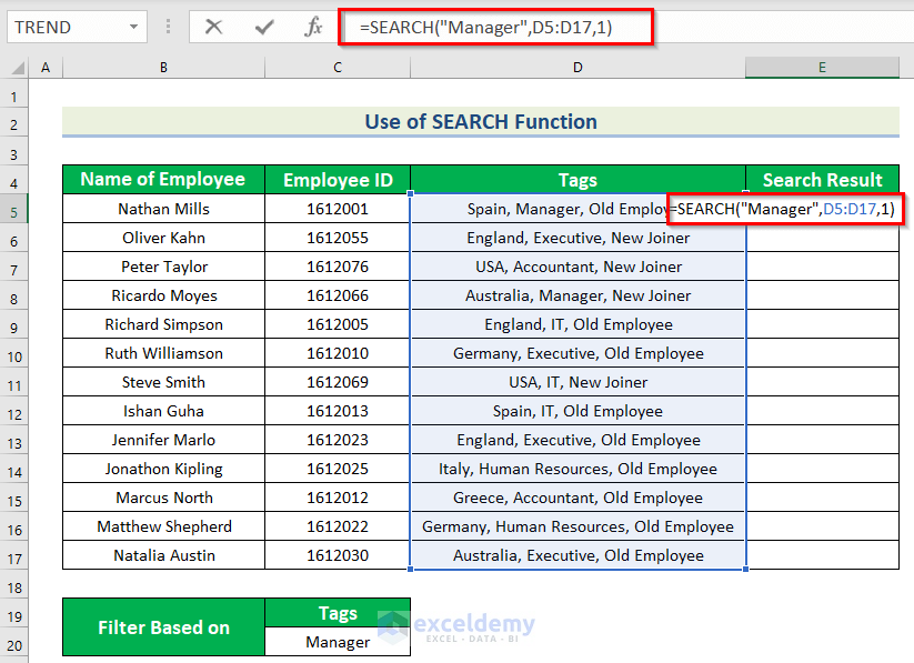
- Press ENTER.
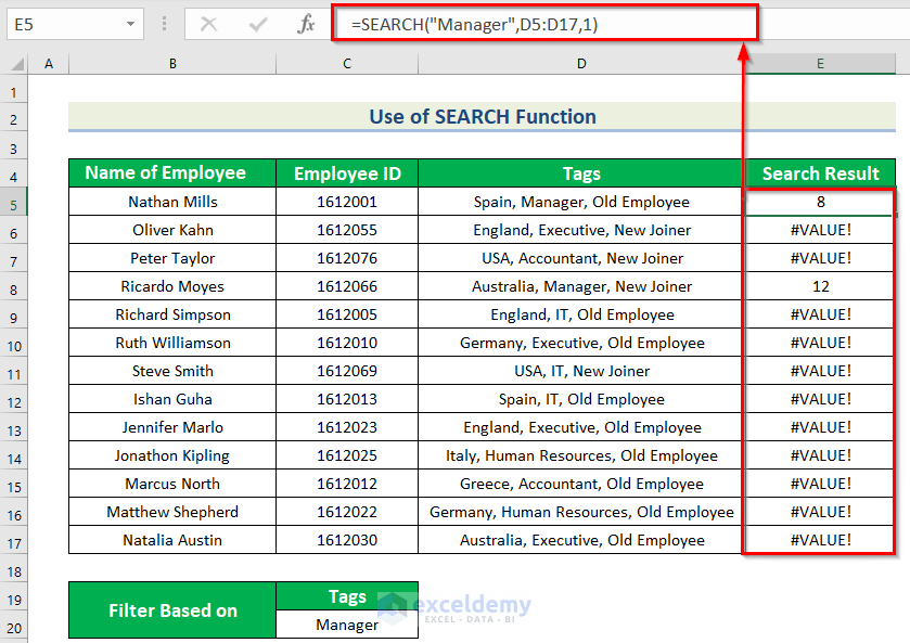
This is the output: a number shows that the cell contains manager.
Read More: How to Filter Tags in Excel
Method 4 – Combining Functions for Multiple Tags
Steps:
- Select E5 to keep the search result.
- Use the formula in E5.
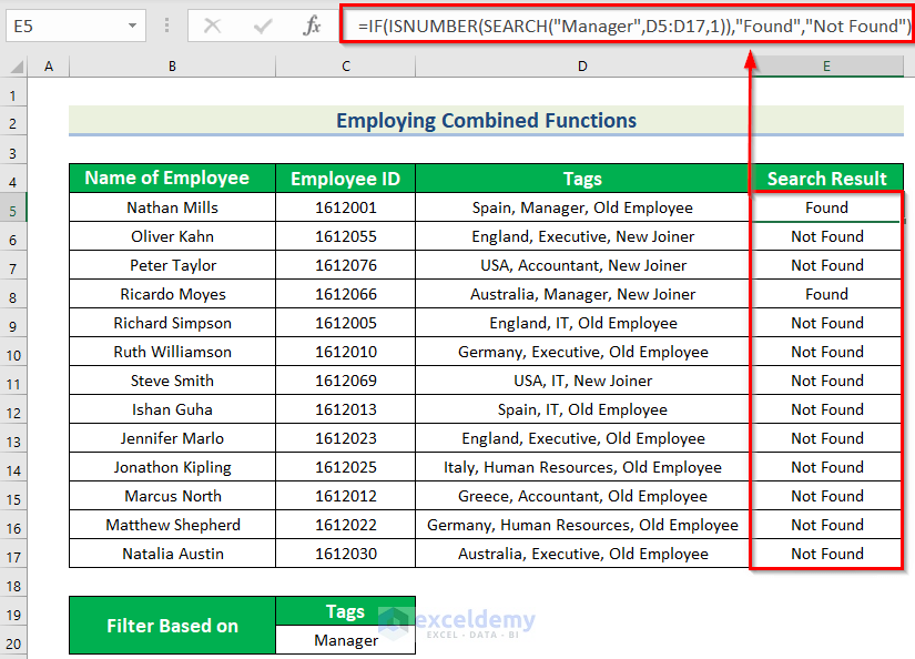
=IF(ISNUMBER(SEARCH("Manager",D5:D17,1)),"Found","Not Found")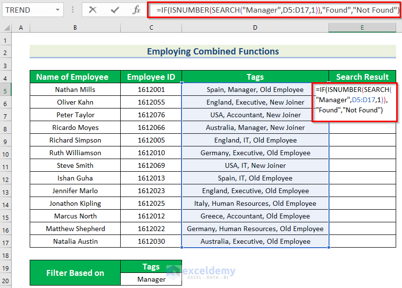
- Press ENTER.
Formula Breakdown
- The SEARCH function searches for “Manager” in D5:D17.
- Output: {8;#VALUE!;#VALUE!;12;#VALUE!;#VALUE!;#VALUE!;#VALUE!;#VALUE!;#VALUE!;#VALUE!;#VALUE!;#VALUE!}.
- The ISNUMBER function checks whether the cell value is a number.
- Output: {TRUE;FALSE;FALSE;TRUE;FALSE;FALSE;FALSE;FALSE;FALSE;FALSE;FALSE;FALSE;FALSE}.
- The IF function performs the same logical test. If the test is TRUE, it returns Found. Otherwise, it returns Not Found. Here, Inverted Comma must be used.
This is the output.
Things to Remember
- To clear the filter option, select any cell within the filtered data and press CTRL+SHIFT+L.
Practice Section
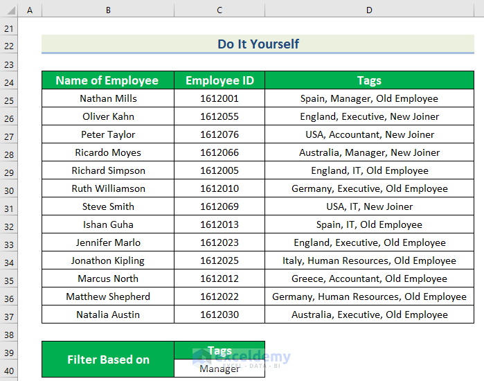
Practice here.
Download Practice Workbook
Download the practice workbook.
Related Articles
<< Go Back to Tags in Excel | Data Analysis with Excel | Learn Excel


