We have a sample dataset with salary sheets of a company called SOFTEKO. Let’s assume the current month is October.
Step 1 – Open Salary Sheet of Previous Month
- Open the salary sheet for the month of September.
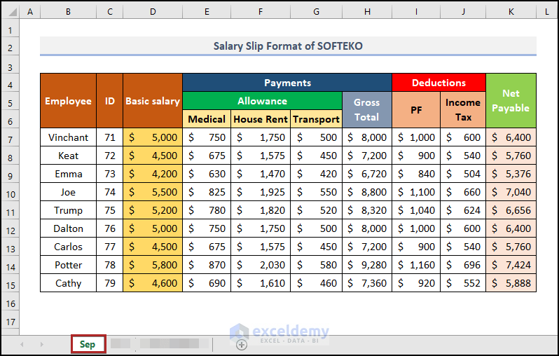
This worksheet contains the Employee name, their corresponding ID, Basic salary, Allowance, Deductions and Net Payable amount for the month of September.
Step 2 – Create Similar Salary Sheet for Ongoing Month
Steps:
- Create a basic outline similar to the sheet of the previous month.
- Enter all the basic salaries in Column D.
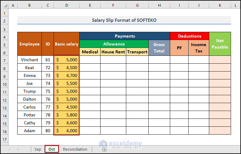
Now, we’ll show how to calculate different allowances. So, see the following.
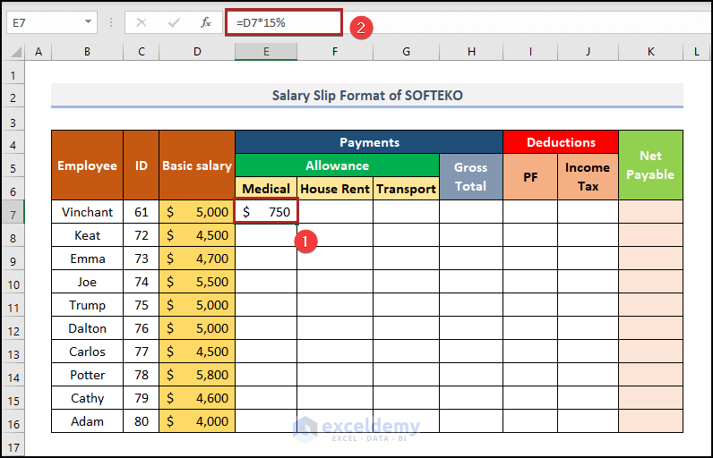
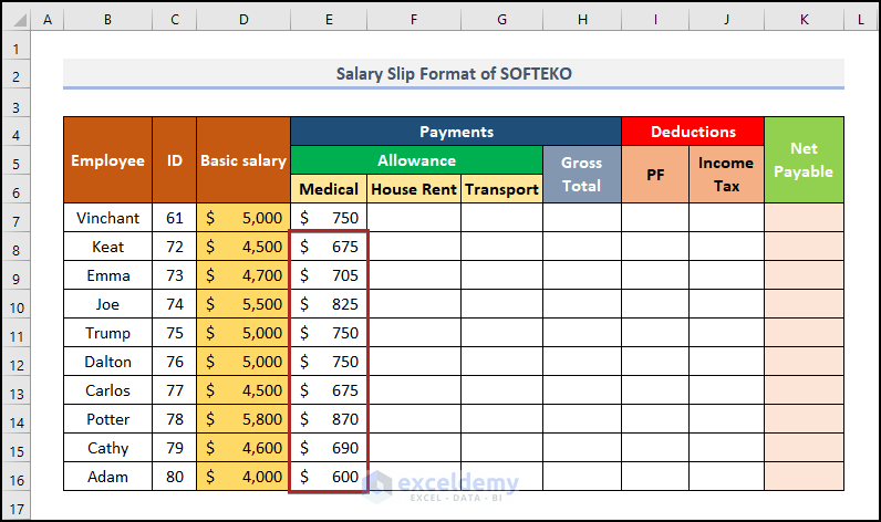
- Select cell E7 and enter the following formula.
=D7*15%
- Press ENTER. It will output the value for medical allowance (we assumed it as 15% of the basic salary).
- Bring the cursor to the bottom right corner of cell E7 to get the Fill Handle tool (it’ll look like a plus (+) sign).
- Double-click on it.
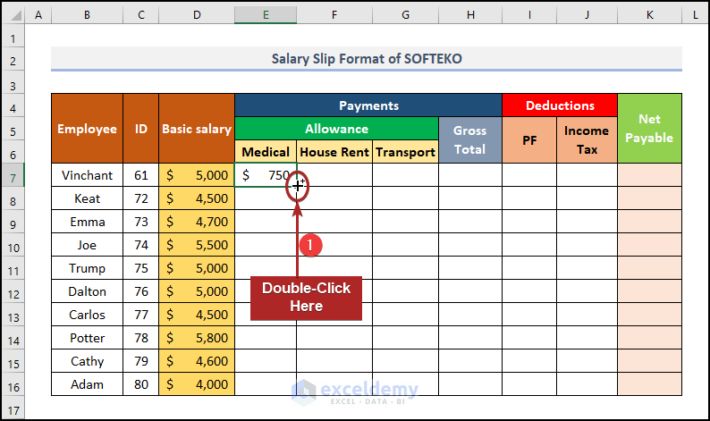
The formula will be copied down to the lower cells in the column.
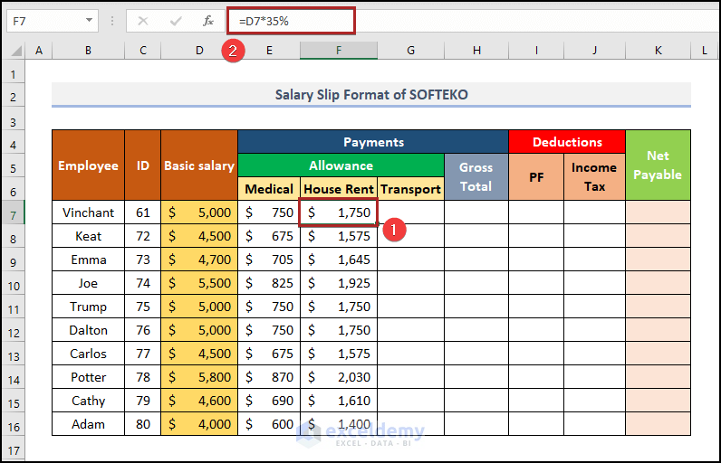
- Consider the House Rent as 35% of the Basic Salary and follow the same process to get the output.
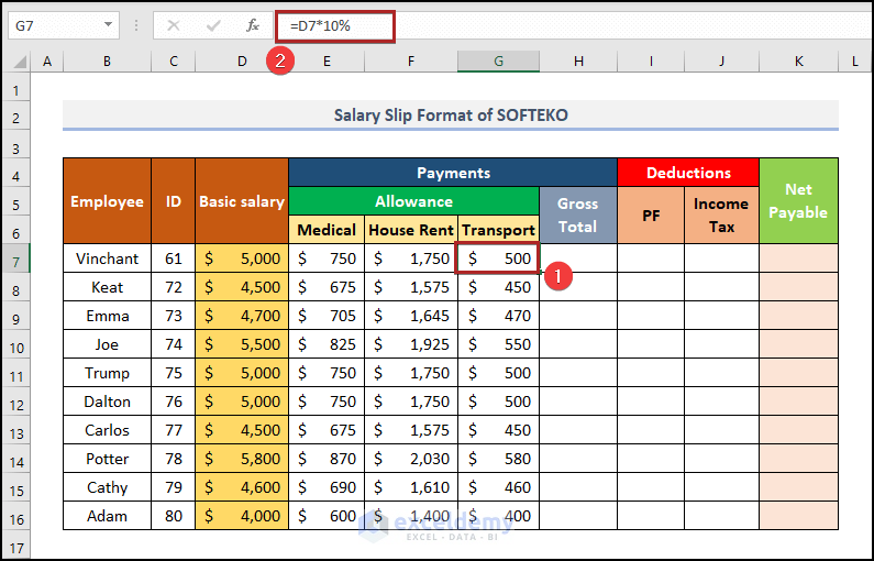
- Consider the Transport allowance as 10% of the basic salary.
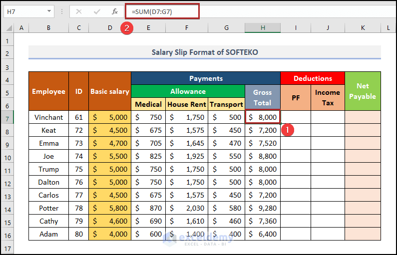
- Used the SUM function to calculate the Gross Total salary.
- Go to cell H7 and insert the formula below.
=SUM(D7:G7)
- Press ENTER.
We need to make deductions from the gross salary. Our deductions are provident fund and income tax. We assumed PF as 20% of basic salary and Income Tax as 12%.
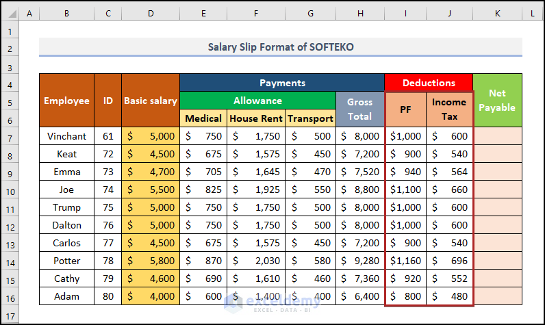
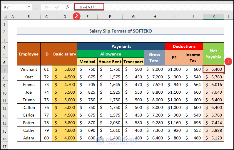
To calculate the Net Payable, subtract the Deductions from the Gross Total.
- Go to cell K7 and add the following formula.
=H7-I7-J7
- Press the ENTER key.
Step 3 – Compare in New Sheet
Steps:
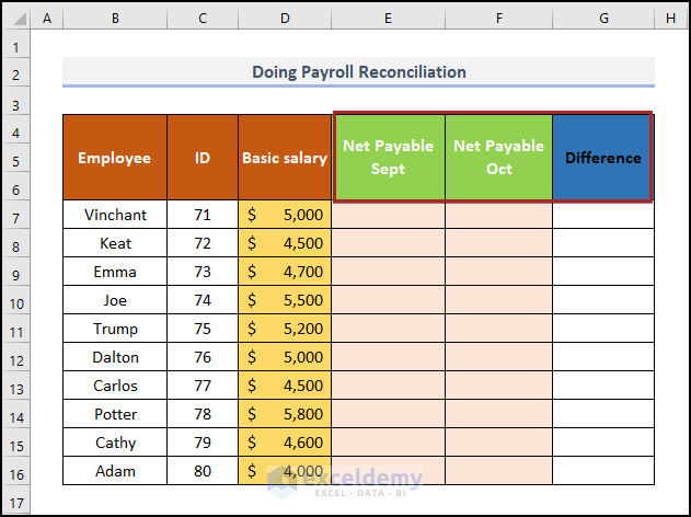
- Create a new worksheet with an outline like the following image.
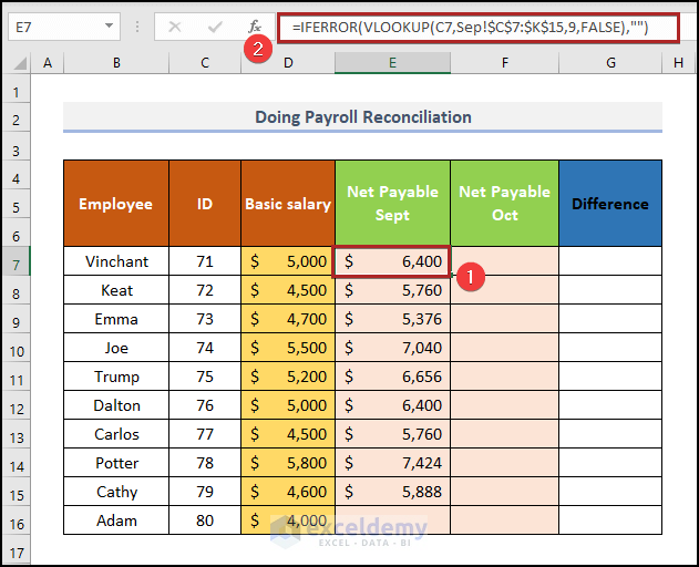
To get the Net Payable amount for the month of September,
- Select cell E7 and paste the following formula.
=IFERROR(VLOOKUP(C7,Sep!$C$7:$K$15,9,FALSE),"")
The VLOOKUP function retrieves the Net Payable from the sheet Sep. The arguments of the function on the Sep worksheet are the following.
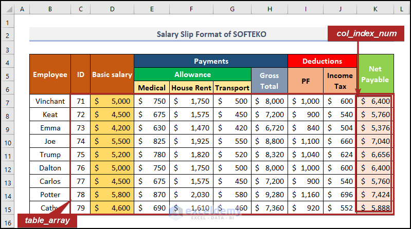
The IFERROR function replaces any error with a blank space.
- Press ENTER.
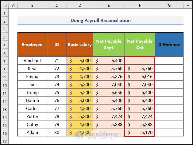
- Follow the same procedure to extract info from the Oct worksheet for the Net Payable Oct column.
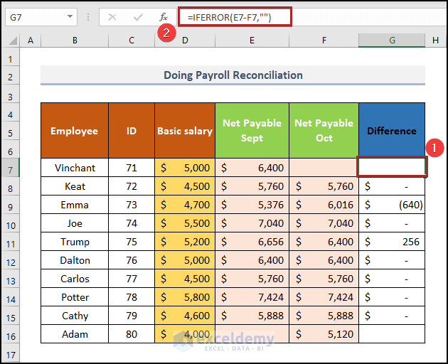
- Go to cell G7 and add the formula below.
=IFERROR(E7-F7,"")
- Press ENTER.
You can see output values in cells F7, G7, G9, G11, E16, and G16, while cells F7 and G7 are blank.
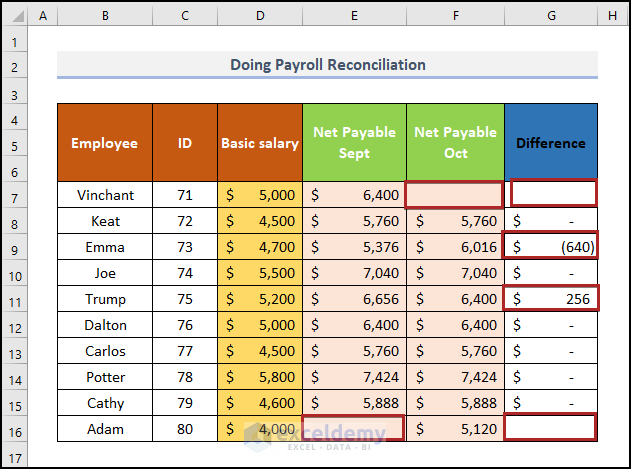
If you go back to the sheet Oct, you can see that there is Net Payable amount visible in cell K7 though we are not getting it in the Reconciliation sheet.
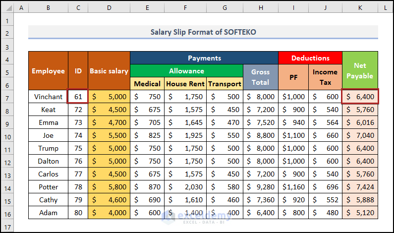
This is because the employee ID isn’t the same in these two worksheets. We entered the wrong ID in Oct sheet. As a result, the formula couldn’t get the result.
The basic salaries of Emma and Trump got changed in the two-salary sheet. And, we didn’t get any Net Payable amount of September in cell E16 as this is a new employee who joined after September.
Read More: Payroll Exercises in Excel
<< Go Back to Formula List | Learn Excel
Get FREE Advanced Excel Exercises with Solutions!

