Example 1 – Sort by Single Color in Excel
Step 1:
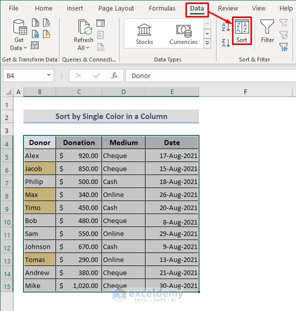
➤ Select the entire table.
➤ Under the Data ribbon, select the Sort option from the Sort & Filter drop-down.
A dialog box will open.
Step 2:
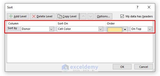
➤ Select Donor from the Sort by list.
➤ Select Cell Color from the Sort On list.
➤ Under the Order bar, choose the only color available (yellow) in the list that will be on top of the selected table.
➤ Press OK.
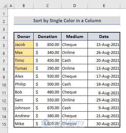
The rows with the highlighted donor names will appear on top.
Read More: How to Add Sort Button in Excel
Example 2 – Sort by Cell Color in Excel (Multiple Layers)
Step 1:
➤ Select the entire table.
➤ Open the Sort dialog box following Example 1.
➤ Select Medium from the Sort by list.
➤ Select Cell Color from the Sort On list.
➤ Under the Order bar, choose an order of color that will be on top of the selected table.
➤ Press OK.
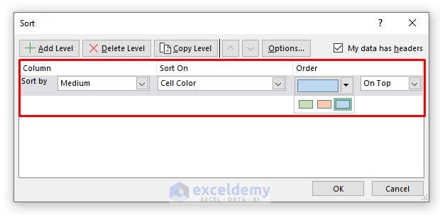
You will see that the table data is sorted by blue rows on top. But the green and orange rows are yet to be sorted. To do this, we have to add another level in the Sort dialog box.
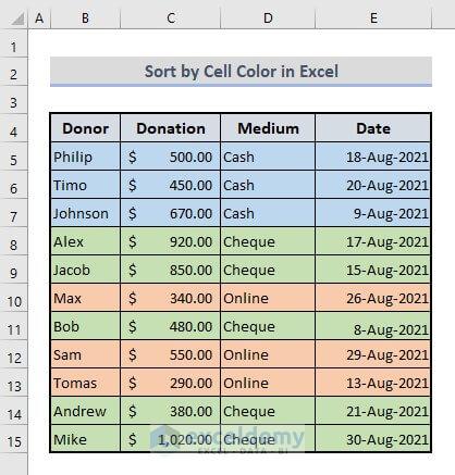
Step 2:
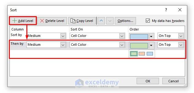
➤ Open the Sort dialog box after selecting the entire table.
➤ Click on Add Level button and you’ll find another row with Sort options.
➤ Select Medium from the Then by list and Cell Color from the Sort on list.
➤ From the Order list, now choose green or orange that you want to see under the blue rows in the table.
➤ Press OK.
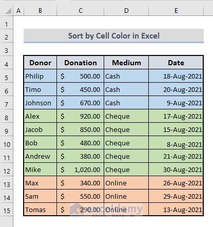
It will organize the dataset with the rows sorted by selected colors on top.
Read More: How to Sort Alphanumeric Data in Excel
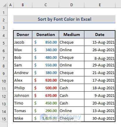
Example 3 – Sort by Font Color in Excel
Steps:
➤ Select the entire table and open the Sort dialog box from the Sort & Filter drop-down under the Data tab.
➤ Under the Column bar, select Donation from the Sort by list.
➤ Select Font Color from the Sort On list.
➤ From the Order list, choose a color that you want to see on top.
➤ Press OK.
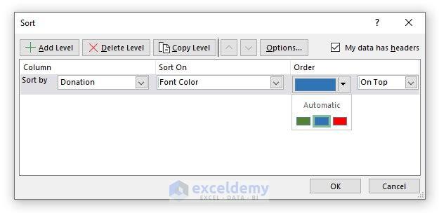
By adding another level for sorting more color fonts, you’ll find a new data table sorted by the color fonts present in a single column.
Read More: How to Remove Sort by Color in Excel
Example 4 – Sort by Icon Color in Excel
Steps:
➤ Select the entire table and open the Sort dialogue box.
➤ Select Date from the Sort by list.
➤ From the Sort On list, select the Conditional Formatting Icon.
➤ Choose a flag color from the Order list which you want to see on top.
➤ Press OK.
![]()
After rearranging the order of all colors available in the table, you should get a modified data table as shown in the following image.
![]()
Read More: Excel Sort and Ignore Blanks
Download Practice Workbook
Related Articles
- How to Sort Data in Excel Using Formula
- How to Use Excel Shortcut to Sort Data
- How to Sort by Ascending Order in Excel
- How to Sort Data in Excel by Value
- How to Sort Data in Alphabetical Order in Excel
- How to Undo Sort in Excel
- How to Remove Sort in Excel
<< Go Back to Sort in Excel | Learn Excel
Get FREE Advanced Excel Exercises with Solutions!

