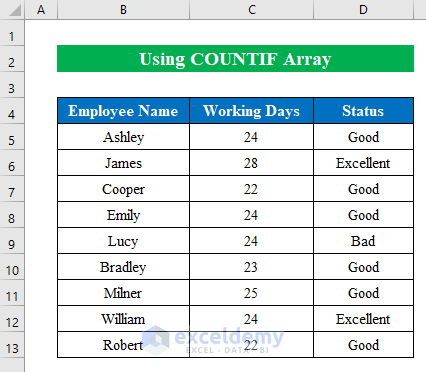
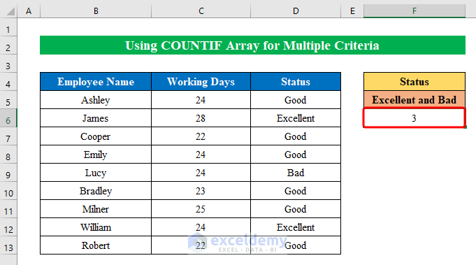
In the dataset below, we have Employee Names, Working Days and employee Status according to performance. We will apply the COUNTIF function with an array to count values.
Method 1 – Utilizing COUNTIF Function to an Array with OR Criteria in Excel
Steps:
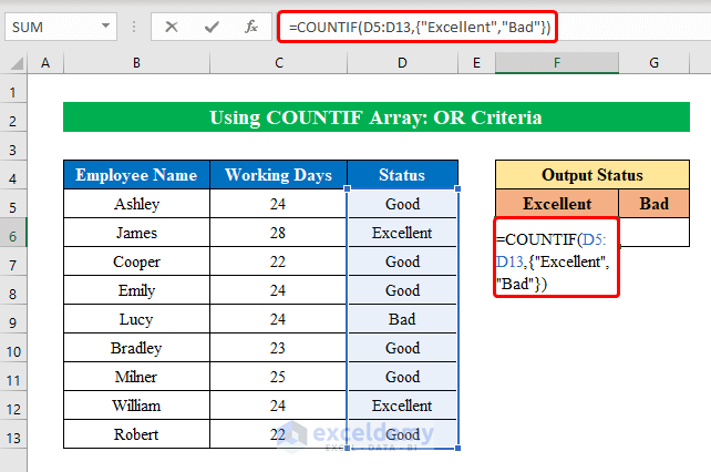
- Choose a cell (F6) and enter the below formula:
=COUNTIF(D5:D13,{"Excellent","Bad"})Where,
- The COUNTIF function counts cells with “Excellent” and “Bad” text values from the given range “D5:D13”.
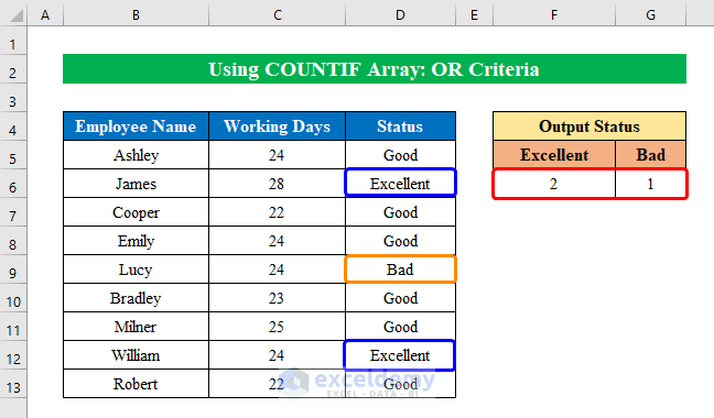
- Press ENTER.
You will get the cell count with your desired text values.
Read More: How to Use COUNTIF for Non-Contiguous Range in Excel
Method 2 – Applying the COUNTIF Function for an Array with Unique Values in Excel
2.1 COUNTIF Function for an Array with Unique Text Values
Steps:
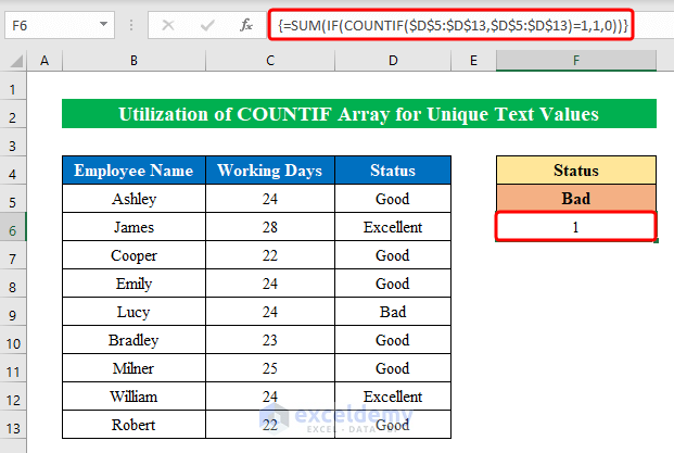
- Choose a cell (F6) and enter the following formula:
=SUM(IF(COUNTIF($D$5:$D$13,$D$5:$D$13)=1,1,0))Where,
- The COUNTIF function will count the occurrences of values from the given range.
- Then, the IF function constructs the results from the COUNTIF It changes the unique values to 1 and the duplicates to 0.
- The SUM function adds up all the counted unique values; thus, the output is 1.
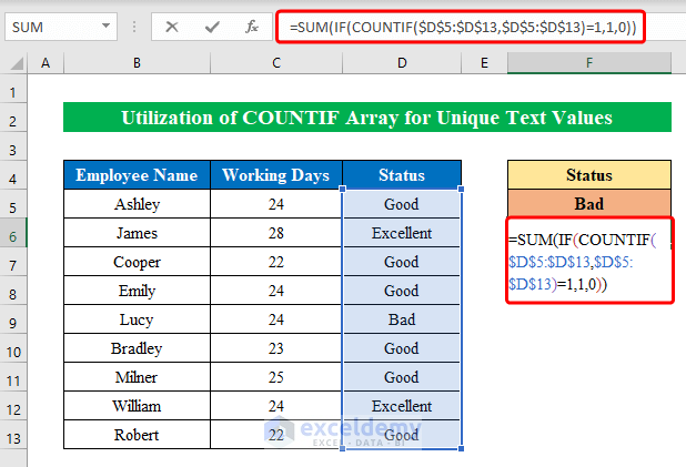
- Click the CTRL+SHIFT+ENTER key from the keyboard to apply an array.
You will get your desired text values counted in the chosen cell.
Read More: COUNTIF Between Two Cell Values in Excel
2.2 COUNTIF Function for an Array with Unique Numeric Values
Steps:
- Select a cell (F5) and enter the following formula into the cell:
=SUM(IF(ISNUMBER($C$5:$C$13)*COUNTIF($C$5:$C$13,$C$5:$C$13)=1,1,0))Where,
- The COUNTIF function counts the number of occurrences from the selected range.
- The ISNUMBER function returns TRUE if the provided value is a number; otherwise, it returns False.
- The IF function converts the unique values to 1 and for duplicates 0.
- The SUM function provides the final output summing up the total counted values.
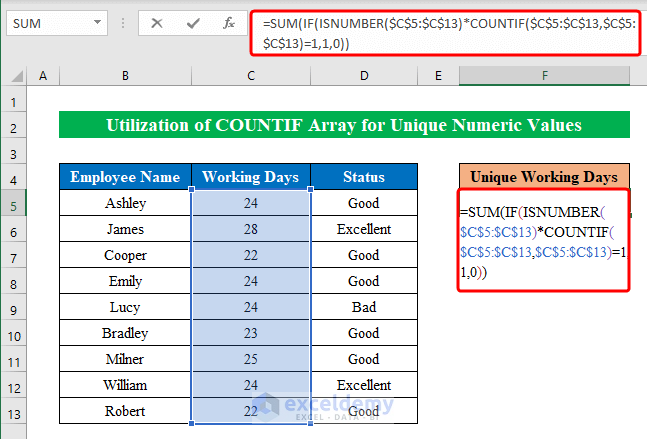
- Press CTRL+SHIFT+ENTER.
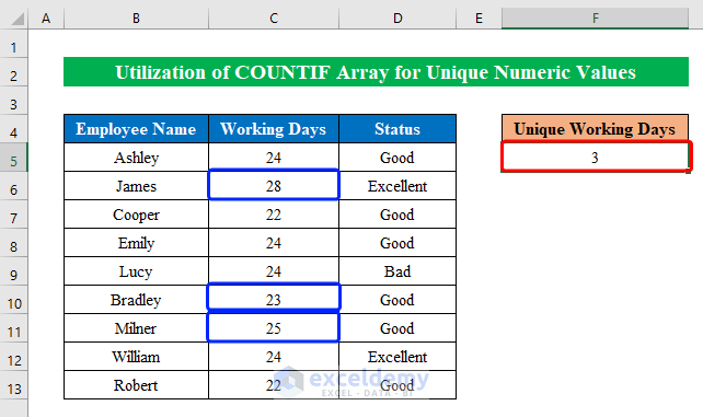
The counted unique values will be displayed.
Read More: Excel COUNTIF to Count Cells Greater Than 1
Method 3 – Using the COUNTIF Function for an Array with Multiple Criteria in Excel
Steps:
- Select a cell (F6) and enter the following formula:
=COUNTIF(D5:D13,"Excellent")+COUNTIF(D5:D13,"Bad")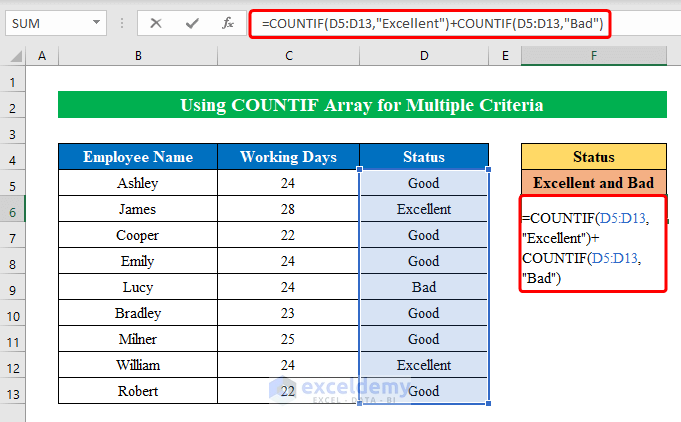
- Press CTRL+SHIFT+ENTER to get the output.
We have successfully counted the cells with desired lookup values from the range.
Read More: How to Calculate Frequency Using COUNTIF Function in Excel
Download the Practice Workbook
Download this workbook to practice.
Related Articles
- How to Use COUNTIF Function to Calculate Percentage in Excel
- COUNTIF Function to Count Cells That Are Not Equal to Zero
- How to Use COUNTIF Function in Excel Greater Than Percentage
- How to Compare Two Columns Using COUNTIF Function
- How to Use Excel COUNTIF Between Time Range
<< Go Back to Excel COUNTIF Function | Excel Functions | Learn Excel
Get FREE Advanced Excel Exercises with Solutions!

