Method 1 – Applying Sort & Filter Feature to Sort by Date in Excel
Steps:
- Select the whole data set by selecting cells B4:D19.
- Go to the Home tab.
- From the Editing group >> select the Sort & Filter option.
- Select the Custom Sort option.

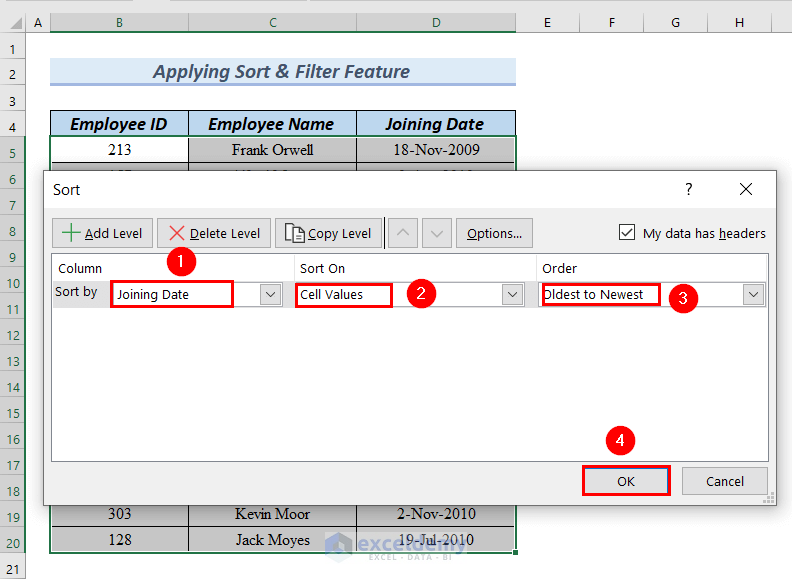
A Custom Sort dialogue box will appear.
- Under the Column option in Sort by, choose the column according to which you want to sort.
We choose Joining Date as we want to sort by date.
- Along with that, under the Sort On option, we choose Cell Values.
- Moreover, under the Order option, we choose Oldest to Newest.
This will sort the Date in ascending order. You can choose any order according to your preference.
- Click OK.
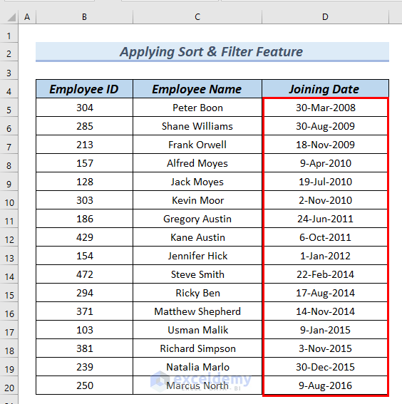
You will find the whole data set sorted according to the joining dates in ascending order.
Method 2 – Using SORT Function to Sort by Date in Excel
Steps:
- We will type the following formula in cell F4.
=SORT(B5:D20,3,1,FALSE)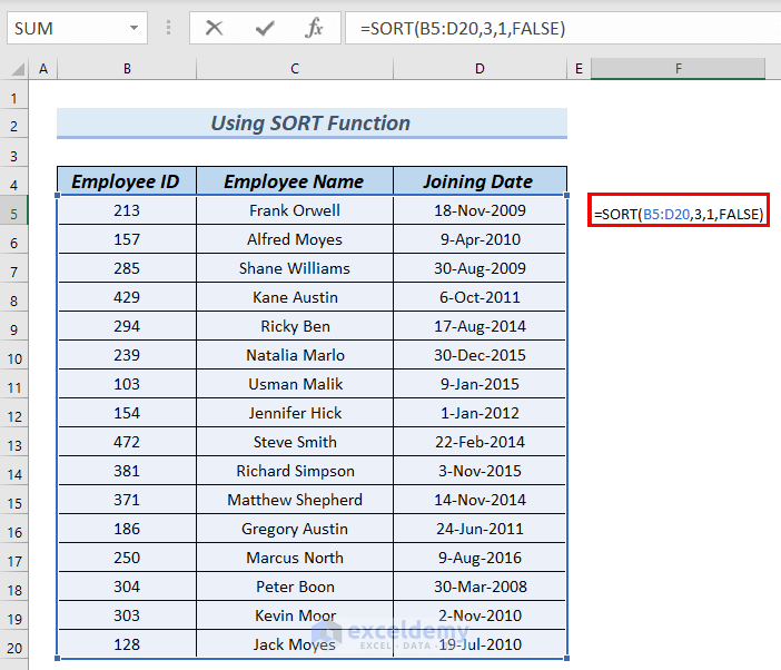
Formula Breakdown
- SORT(B5:D20,3,1,FALSE) →The SORT function sorts the values of a range of cells.
- B5:D20 → is the array.
- 3 → is sort_index.
- 1 → indicates ascending order.
- FALSE → indicates row-wise.
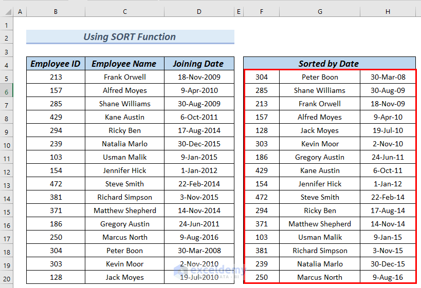
- Press ENTER.
We sorted according to the joining dates in ascending order.
Method 3 – Use of SORTBY Function to Sort by Date in Excel
Steps:
- Type the following formula in cell F5.
=SORTBY(B5:C20,D5:D20,1)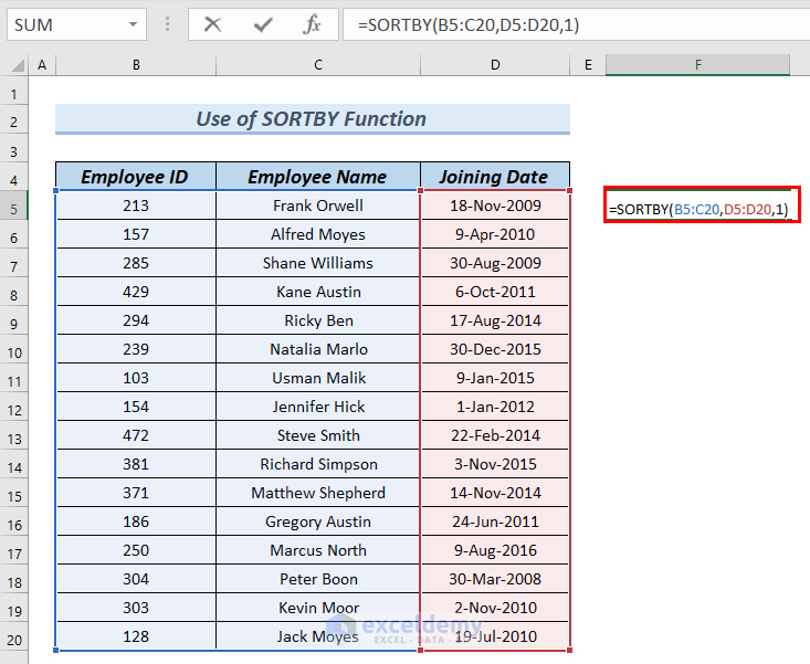
Formula Breakdown
- SORTBY(B5:C20,D5:D20,1) → the SORTBY function sorts the values in a range of cells based on values in a specific array.
- B5:C20 → is the array.
- D5:D20 → is the by_array.
- 1 → indicates ascending order.
- Press ENTER.
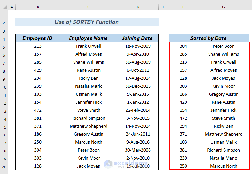
The Employee IDs and Employee Names are sorted in ascending order, according to the Joining Dates.
Method 4 – Using SORTBY and MONTH Functions to Sort by Months
Steps:
- Type the following formula in cell F5.
=SORTBY(B5:D20,MONTH(D5:D20),1)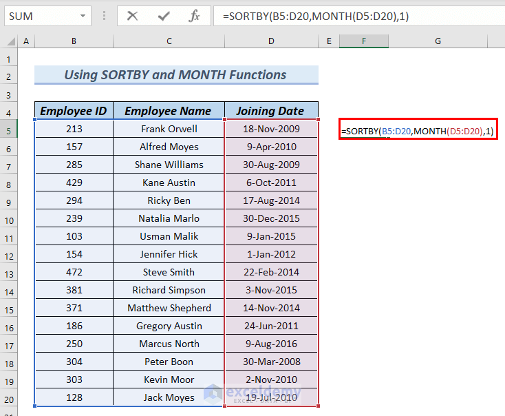
Formula Breakdown
- SORTBY(B5:D20,MONTH(D5:D20),1) → the SORTBY function sorts the values in a range of cells based on values in a specific array.
- B5:D20 → is the array.
- MONTH(D5:D20) → the MONTH function returns the month number of the joining dates.
- 1 → indicates ascending order.
- SORTBY(B5:D20,MONTH(D5:D20),1) → sorts the data set B5:D20 according to the months of the dates D5:D20, in ascending order.
- Press ENTER.
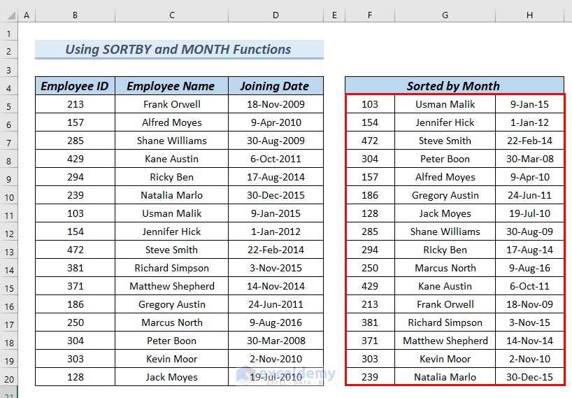
Find the data set sorted by the months of the joining dates of the employees in ascending order.
Method 5 – Applying SORTBY and DAY Functions to Sort by Day in Excel
Steps:
- Type the following formula in cell F5.
=SORTBY(B5:D20,DAY(D5:D20),1)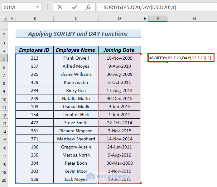
Formula Breakdown
- SORTBY(B5:D20,DAY(D5:D20),1) → the SORTBY function sorts the values in a range of cells based on values in a specific array.
- B5:D20 → is the array.
- DAY(D5:D20) → the DAY function returns the date of a range of cells.
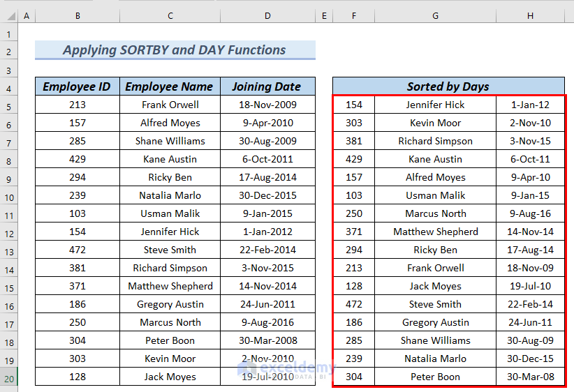
- SORTBY(B5:D20,DAY(D5:D20),1) → sorts the data set B5:D20 according to the days of the dates D5:D20, in ascending order.
- Press ENTER.
You can see the result in cells F5:H19.
Method 6 – Using SORTBY and YEAR Functions to Sort by Years in Excel
Steps:
- Type the following formula in cell F5.
=SORTBY(B5:D20,YEAR(D5:D20),1)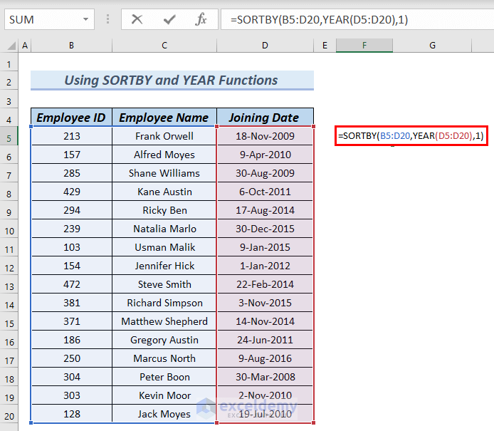
Formula Breakdown
- SORTBY(B5:D20,YEAR(D5:D20),1) → the SORTBY function sorts the values in a range of cells based on values in a specific array.
- B5:D20 → is the array.
- YEAR(D5:D20) → the YEAR function returns the year based on a date.
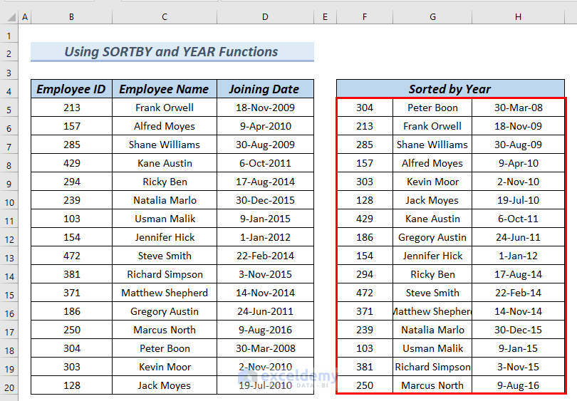
- SORTBY(B5:D20,YEAR(D5:D20),1) → sorts the data set B5:D20 according to the year of the dates D5:D20, in ascending order.
- Press ENTER.
Get the data set sorted according to the years in ascending order.
Method 7 – Using SORTBY, DAY, and MONTH Functions in Excel
Steps:
- Type the following formula in cell F5.
=SORTBY(B5:D20,MONTH(D5:D20)+(DAY(D5:D20)/100))
Formula Breakdown
- SORTBY(B5:D20,MONTH(D5:D20)+(DAY(D5:D20)/100)) → the SORTBY function sorts the values in a range of cells based on values in a specific array.
- B5:D20 → is the array.
- MONTH(D5:D20) → the MONTH function returns the month number of the joining dates
- DAY(D5:D20) → the DAY function returns the date of a range of cells.
- MONTH(D4:D19)+(DAY(D4:D19)/100) → becomes the by_array of the formula.
- SORTBY(B4:D19,MONTH(D4:D19)+(DAY(D4:D19)/100)) → sorts the data set B5:D20 according to only the months and days of the dates D5:D20, in ascending order.
- Press ENTER.
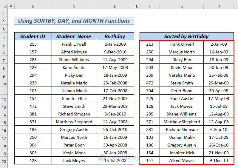
Get the data set sorted by the ascending birthdays.
Method 8 – Applying INDEX, MATCH, ROW, and RANK Functions
In this method, we will use the combination of the INDEX, MATCH, ROW, and RANK functions to sort by date in Excel. This method is helpful if you do not have an Office 365 subscription,
The first data set, but a new column Salary has been inserted between the Employee Name and Joining Date.
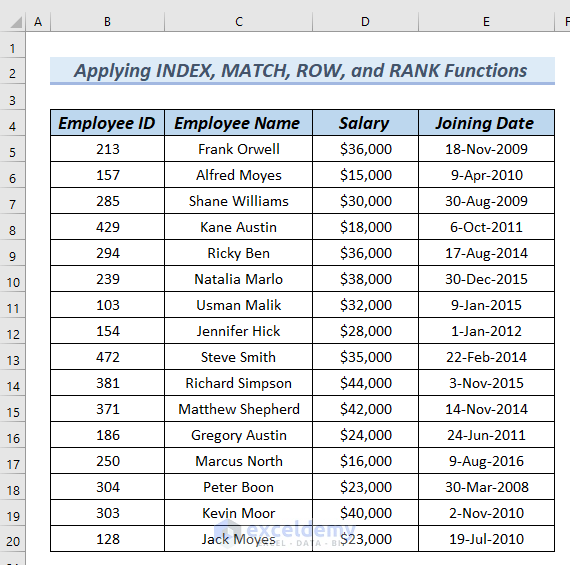
If we want to sort not all the columns, only the Employee ID, Employee Name, and Joining Date, according to the Joining Date?
You can not execute this using the SORT or SORTBY function of Excel.
Using the SORT and SORTBY functions, you can only sort the adjacent columns, not the non-adjacent ones.
That means you can sort the Employee Name, Salary, and Joining Date. Or, the Employee ID, Employee Name, and Salary. Or, the Name and Salary.
But not the Employee ID, Employee Name, and Joining Date.
You can use a combination of the INDEX, MATCH, ROW, and RANK functions of Excel to sort the columns that are not adjacent.
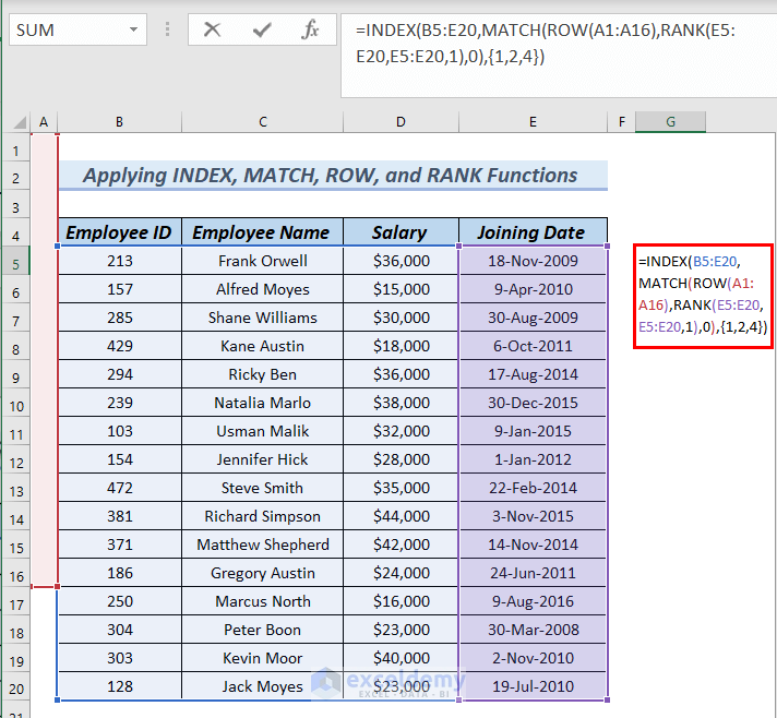
- To sort Employee ID, Employee Name, and Joining Date according to the Joining Date, in ascending order, we will type the following formula in cell G5.
=INDEX(B5:E20,MATCH(ROW(A1:A16),RANK(E5:E20,E5:E20,1),0),{1,2,4})[This is an Array Formula. So do not forget to press CTRL+SHIFT+ENTER unless you are in Office 365.]
Formula Breakdown
- ROW(A1:A16) → the ROW function returns an array with the numbers from 1 to 16, like {1, 2, 3, …, 16}. We have taken from 1 to 16 because each of my columns has 16 values (B5:B20).
- RANK(E5:E20,E5:E20,1) → the RANK function returns an array containing the rank of each cell in column E5:E20 in ascending order. To get in descending order, use 0 in place of 1.
- MATCH(ROW(A1:A16),RANK(E5:E20,E5:E20,1),0) → the MATCH function returns the position of each of the numbers in the array {1, 2, 3, …, 16} in the array returned by the RANK
- INDEX(B4:E19,MATCH(ROW(A1:A16),RANK(E4:E19,E4:E19,1),0),{1,2,4}) → the INDEX function returns the columns 1,2 and 4 (ID, name, and joining dates) from the range B5:E20 in ascending order.
- Press ENTER.
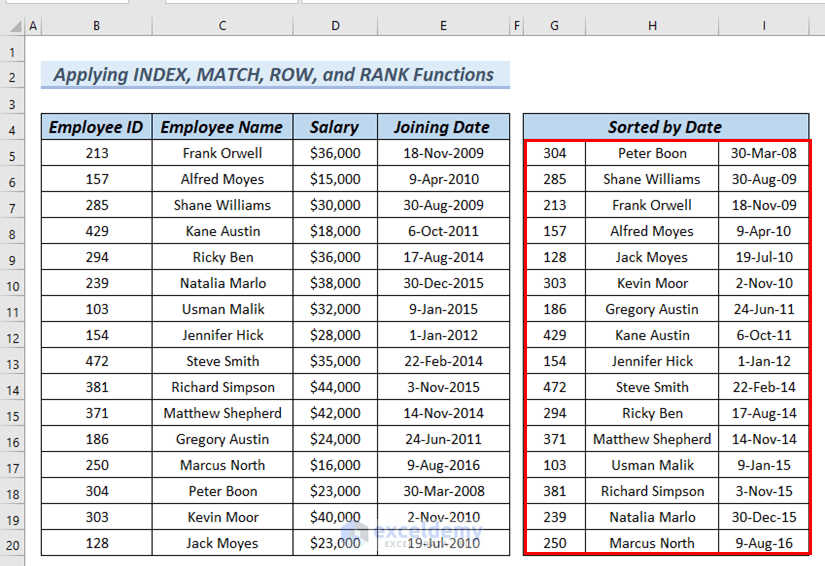
You will find the Employee ID, Employee Name, and Joining Date sorted in ascending order, according to the Joining Date.
Method 9 – Applying VBA to Sort by Date in Excel
Steps:
- Press ALT+F11 to bring out the VBA editor window.
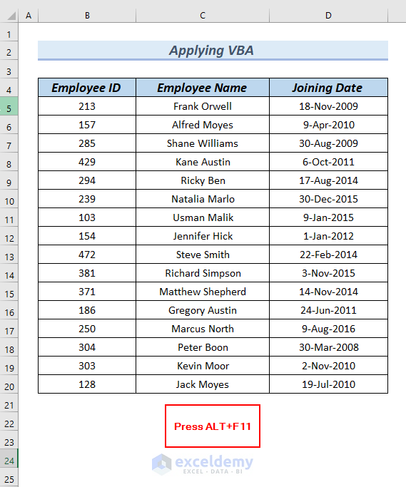
At this moment, a VBA editor window will appear.
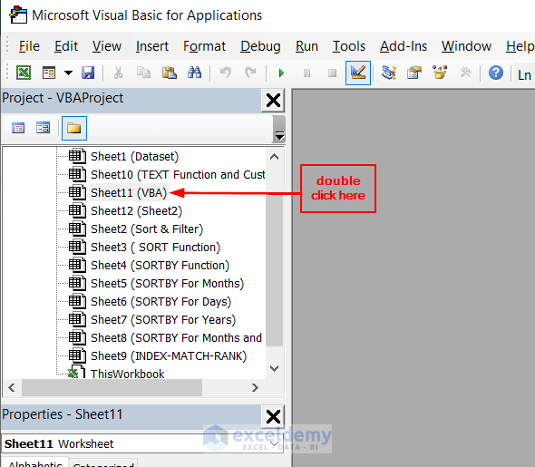
- Double-click on Sheet11 (VBA).
- Type the following code in the editor window.
Private Sub Worksheet_Change(ByVal Target As Range)
   On Error Resume Next
   Range("B4").Sort Key1:=Range("D5"), _
     Order1:=xlAscending, Header:=xlYes, _
     OrderCustom:=1, MatchCase:=False, _
     Orientation:=xlTopToBottom
End Sub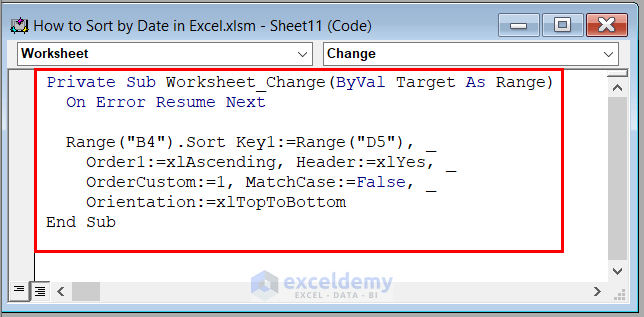
Code Breakdown
- Declare a Private Sub since we want the code to run in a specific sheet.
- Take the starting cell B4 of our dataset in the first Range.
- Take the starting date cell D5 of our dataset in the second Range.
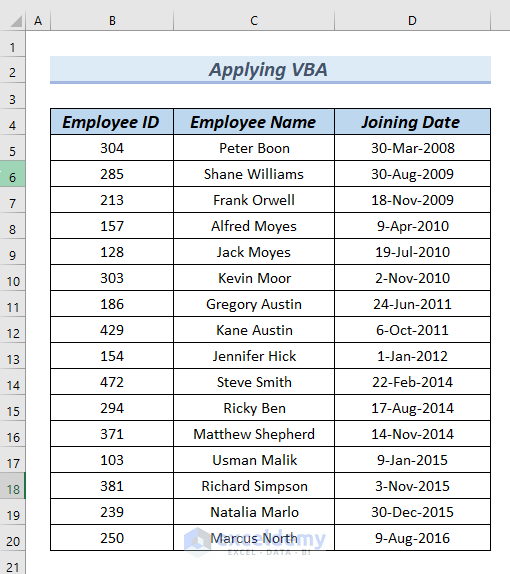
We close the VBA editor window and go back to our worksheet.
See that the dataset has been sorted by date.
Download Practice Workbook
You can download the Excel file from the link below and practice while reading this article.
How to Sort by Date in Excel: Knowledge Hub
<< Go Back to Sort in Excel | Learn Excel
Get FREE Advanced Excel Exercises with Solutions!

