Method 1 – Using Excel Power Query Editor to Combine 2 Columns
Steps:
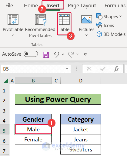
- Select cell B5 in the Gender column.
- Go to the Insert tab.
- Select Table.
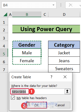
- A prompt will open on the screen.
- Select B5:B6 as the table range and click.
- The range will be converted into a table.
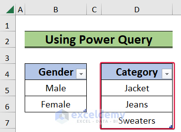
- Repeat the process for the Category column and turn it into a table.
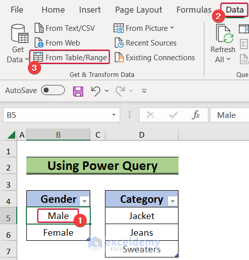
- Select cell B5 and go to the Data tab.
- From the Data tab, select From Table/Range.
- The column will open in the Power Query window.
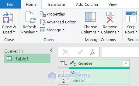
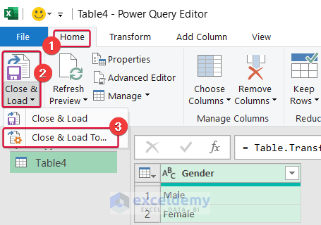
- In the Power Query window, go to the Home tab.
- Select Close & Load To from the Close & Load option.
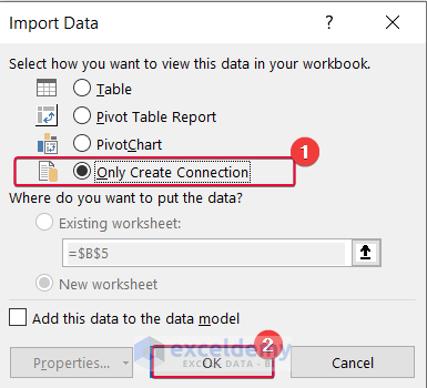
- A prompt will open on the screen.
- Choose the Only Create Connection option.
- Click OK.
- A connection table sign will appear on the right side of the sheet.
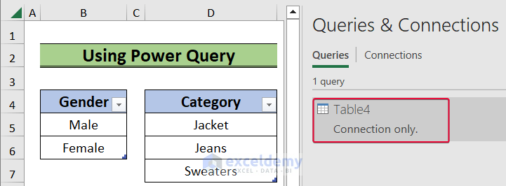
- Repeat the same steps for the Category table.
There will be two table connections.
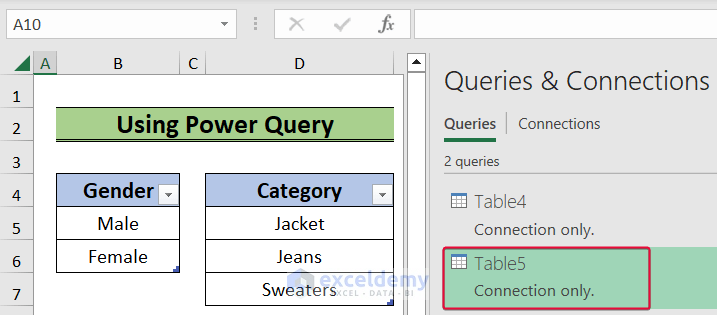
- Choose Table4.
- The Power Query window will open.
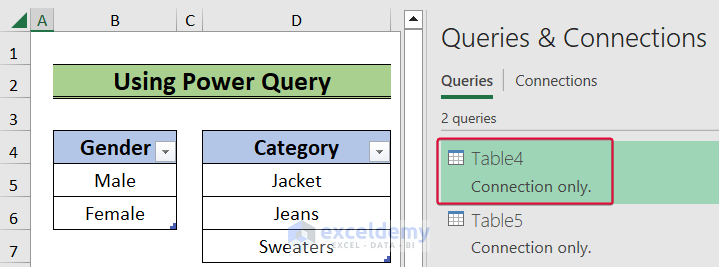
- Go to the Add Column.
- Select Custom Column.
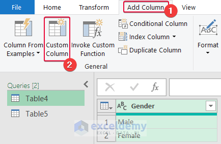
- In the Custom Column prompt, enter Table5.
- Click OK.
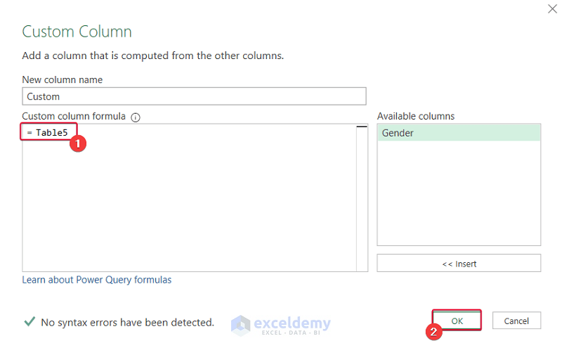
- The Custom column will be added beside the Gender column.
- Select the double arrow sign in the top right corner of the column.

- Select OK.
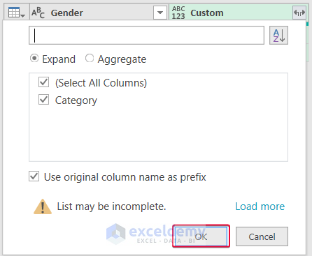
- The Category column will appear beside the Gender column.
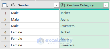
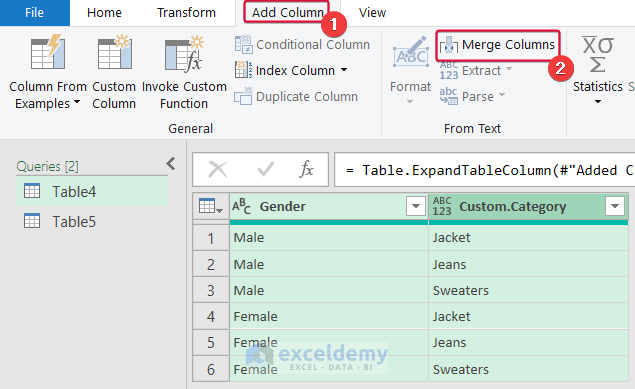
- Go to the Add Column tab.
- Select Merge Columns.
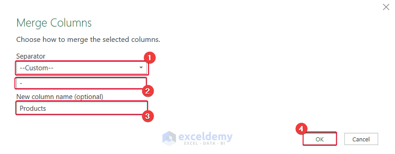
- A prompt will open on the screen.
- Select Custom.
- Type “-” as the separator.
- Rename the merged column as Products.
- Choose OK.
We will have all the combinations of the 2 columns in Power Query.

- Open a new worksheet.
- Go to the Data tab.
- Select Queries & Connections.
- The list of tables will appear on the right side of the sheet.

- Choose cell B4.
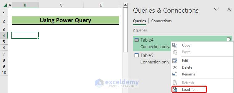
- Right-click on one of the tables.
- From the available options, select Load To.
- A prompt will open on the screen.
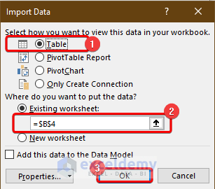
- Select Table.
- Select cell B4 as the cell to insert the table.
- Click OK.
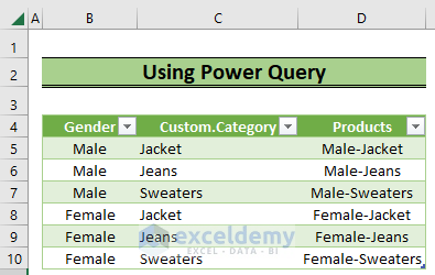
We will get all the combinations of the 2 columns.
Method 2 – Applying Combined Excel Functions
Steps:
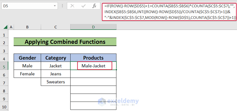
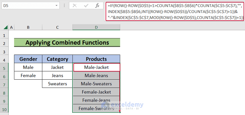
- Click on cell D5 and enter,
=IF(ROW()-ROW($D$5)+1>COUNTA($B$5:$B$6)*COUNTA($C$5:$C$7),"", INDEX($B$5:$B$6,INT((ROW()-ROW($D$5))/COUNTA($C$5:$C$7)+1))&"-"&INDEX($C$5:$C$7,MOD(ROW()-ROW($D$5),COUNTA($C$5:$C$7))+1))- Press Enter.
Formula Breakdown
- ROW()-ROW($D$5)+1>COUNTA($B$5:$B$6)*COUNTA($C$5:$C$7): Here, the ROW() returns the value of the row of the D5 cell which is So as the ROW($D$5). Now, the formula becomes 5-5+1>COUNTA($B$5:$B$6)*COUNTA($C$5:$C$7). The COUNTA($B$5:$B$6) and COUNTA($C$5:$C$7) return the number of non-empty cells in the range B5:B6 and C5:C7, which are 2 and 3 respectively. So the expression becomes 1>2*3 or 1>6, which is False.
- Output: False
- INDEX($B$5:$B$6,INT((ROW()-ROW($D$5))/COUNTA($C$5:$C$7)+1)): The (ROW()-ROW($D$5) returns The COUNTA($C$5:$C$7) expression counts the number of non-empty cell in the C5:C7 range and returns 3. So, the expression becomes INDEX($B$5:$B$6,INT(0/3+1)) and will become INDEX($B$5:$B$6,INT(0+1)) or INDEX($B$5:$B$6,INT(1)) . The INT function will return 1. The final expression will be INDEX($B$5:$B$6,1). Finally, the INDEX function will return the 1st value of the B5:B6 range, which is Male.
- Output: Male
- INDEX($C$5:$C$7,MOD(ROW()-ROW($D$5),COUNTA($C$5:$C$7))+1)): The MOD(ROW()-ROW($D$5),COUNTA($C$5:$C$7))+1 will become MOD(0,3)+1. The MOD function will return the remainder of the division between 0 and 3 which is So, the INDEX($C$5:$C$7,MOD(ROW()-ROW($D$5),COUNTA($C$5:$C$7))+1)) becomes INDEX($C$5:$C$7,0+1)) or INDEX($C$5:$C$7,1)). Thus, the expression will return the first value of the cell range C5:C7 and that will be Jacket.
- Output: Jacket
- IF(ROW()-ROW($D$5)+1>COUNTA($B$5:$B$6)*COUNTA($C$5:$C$7),””, INDEX($B$5:$B$6,INT((ROW()-ROW($D$5))/COUNTA($C$5:$C$7)+1))&”-“&INDEX($C$5:$C$7,MOD(ROW()-ROW($D$5),COUNTA($C$5:$C$7))+1)): This expression becomes IF(False,#NA, “Male” &”-“& “Jacket”). So, the expression is asking to concatenate the Male , – , and Jacket if the condition is
- Output: Male-Jacket
- We will have the first combination of the two columns.
- Drag the cursor down to autofill the rest of the cells.
Method 3 – Using Helper Columns and Combined Functions
Steps:
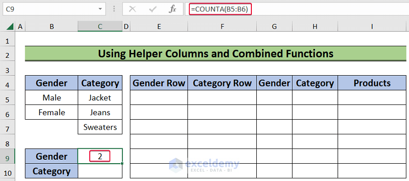
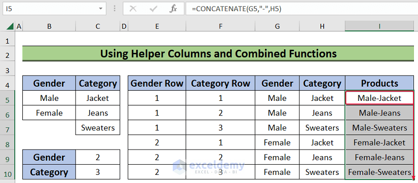
- Choose cell C9 and enter the following formula:
=COUNTA(B5:B6)- Press Enter.
- We will have the counting of the values in the Gender column.
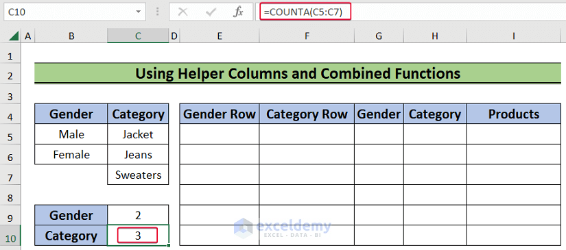
- Select cell C10 and enter the following formula:
=COUNTA(C5:C7)- Press Enter.
- We will get the number of values under the Category column.
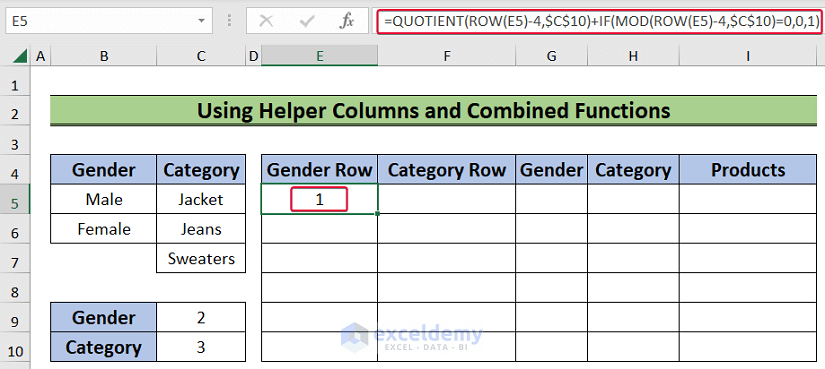
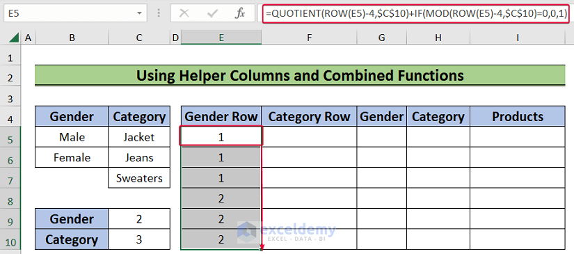
- Choose cell E5 and enter the following formula:
=QUOTIENT(ROW(E5)-4,$C$10)+IF(MOD(ROW(E5)-4,$C$10)=0,0,1)- Press Enter.
Formula Breakdown
- QUOTIENT(ROW(E5)-4,$C$10): The ROW(E5)-4 expression will become 5-4 or So the overall expression be QUOTIENT(1,$C$10) or QUOTIENT(1,3). The QUOTIENT function will return the integer part of the division of 1 by 3 which is 0.
- Output: 0
- IF(MOD(ROW(E5)-4,$C$10)=0,0,1): The ROW(E5)-4 expression will return The MOD(ROW(E5)-4,$C$10) will become MOD(1,3) which returns 1. So, the overall expression will be IF(1=0,0,1) or IF(False,0,1). Finally, the formula will return 1.
- Output: 1
- QUOTIENT(ROW(E5)-4,$C$10)+IF(MOD(ROW(E5)-4,$C$10)=0,0,1): The entire expression will become 0+1 or
- Output: 1
- We will assign the row number for the first value of the Gender column.
- Drag the cursor down and autofill the rest of the cells.
- Click on cell F5 and enter the following formula:
=COUNTIF($E$5:E5,E5)- Press Enter.
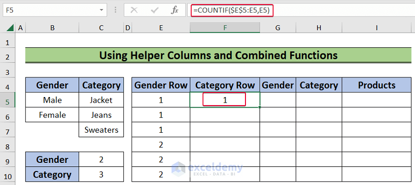
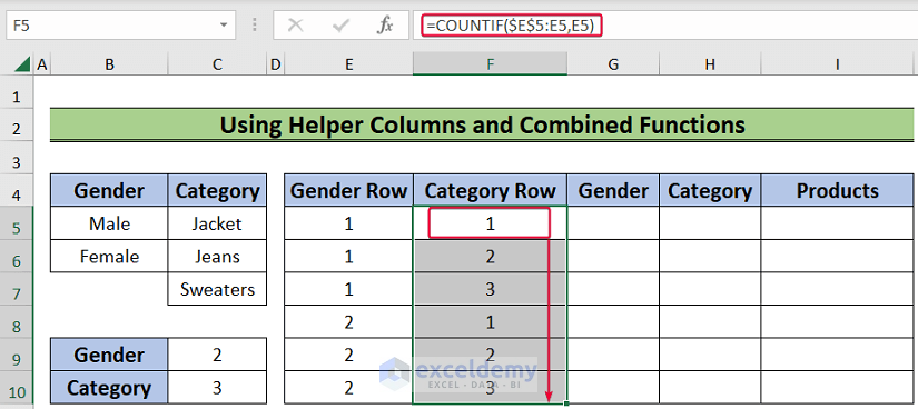
- We will get the row number for the first value of the Category column.
- Drag the cursor down to autofill.
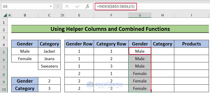
- Choose cell G5 and enter the following formula:
=INDEX($B$5:$B$6,E5)- Press Enter.
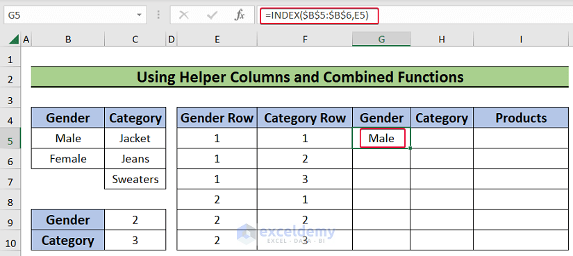
- We will have the first value of the Gender column associated with the value in the Gender Row.
- Drag the cursor to autofill the rest of the cells.
- Choose cell H5 and enter the following formula:
=INDEX($C$5:$C$7,F5)- Press Enter.
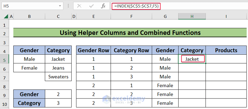
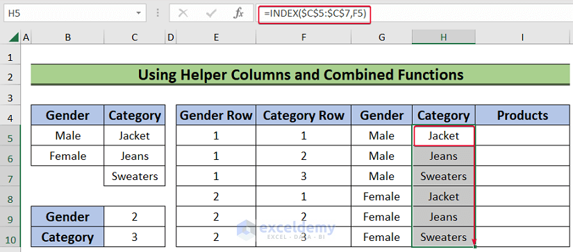
- We will have the first value of the Category column associated with the value in the Category Row.
- Drag the cursor down to the last cell to autofill.
- Choose cell I5 and enter the following formula:
=CONCATENATE(G5,"-",H5)- Press Enter.
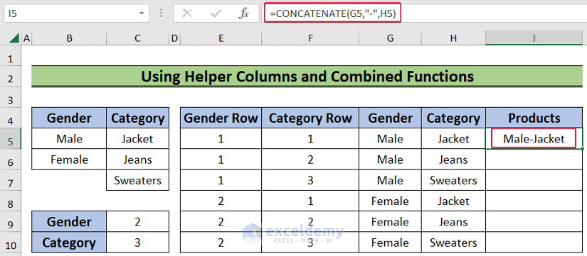
- We will have our first combination of the 2 columns.
- Drag the cursor to autofill the rest of the cells.
Method 4 – Applying VBA Code
Steps:
- Go to the Developer tab.
- Select the Visual Basic tab.
- A new window will open on the screen.

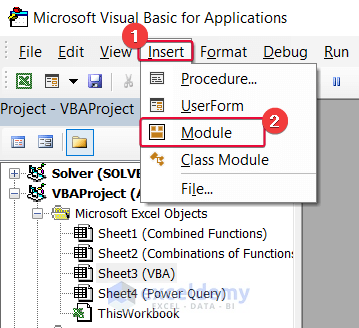
- From the Visual Basic window, select Insert.
- Choose Module from the drop-down list.
- A new module will appear.
- Enter the following formula and save it:
Sub AllCombinationsTwoColumns()
Dim am_r1, am_r2 As Range
Dim am_r  As Range
Dim am_str As String
Dim am_int1, am_int2 As Integer
Dim am_str1, am_str2 As String
Set am_r1 = Range("B5:B6")
Set am_r2 = Range("C5:C7")
am_str = "-"
Set am_r = Range("D5")
For am_int1 = 1 To am_r1.Count
    am_str1 = am_r1.Item(am_int1).Text
    For am_int2 = 1 To am_r2.Count
        am_str2 = am_r2.Item(am_int2).Text
        am_r.Value = am_str1 & am_str & am_str2
        Set am_r = am_r.Offset(1, 0)
       Next
    Next
End Sub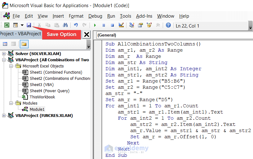
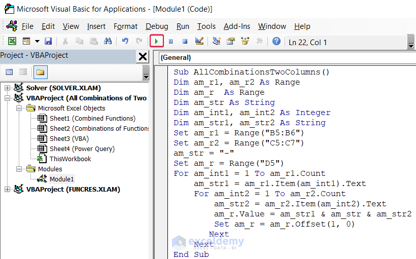
- Run the code by clicking on the triangular-shaped green button.
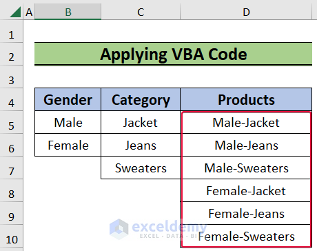
- We will have all the combinations of 2 columns in the D5:D10 cell range.
Download the Practice Workbook
You can download the practice workbook here.
Related Articles
- How to Sum All Possible Combinations in Excel
- How to Find Combinations Without Repetition in Excel
- How to Apply All Combinations of 3 Columns in Excel
- How to Create All Combinations of 4 Columns in Excel
- How to Show All Combinations of 5 Columns in Excel
- How to Create All Combinations of 6 Columns in Excel
<< Go Back to Excel COMBIN Function | Excel Functions | Learn Excel
Get FREE Advanced Excel Exercises with Solutions!

